Download
1 / 42
420 likes | 576 Views
Lecture 11 Associative Containers. Road Map Associative Container Impl . Unordered ACs Hashing Collision Resolution Open Addressing Separate Chaining Ordered ACs Balanced Search Trees 2-3-4 Trees Red-Black Trees. Road Map. Implementing Associative Containers (ACs)

E N D
Lecture 11 Associative Containers • Road Map • Associative Container Impl. • Unordered ACs • Hashing • Collision Resolution • Open Addressing • Separate Chaining • Ordered ACs • Balanced Search Trees • 2-3-4 Trees • Red-Black Trees
Road Map • Implementing Associative Containers (ACs) • Hash Tables (Unordered ACs; Ch. 5) • 2-3-4 Trees (Ordered; 4) • Red-Black Trees (Ordered; 12) • Inheritance and Polymorphism revisited • Heaps (PQ implementation: 6) • Divide and Conquer Algs. • Mergesort, Quicksort (7) • Intro to Graphs (9) • Representations • Searching • Topological Sorting, Shortest Path
Associative Containers • Categories • Ordered (OAC) – iterate through elements in key order • Unordered (UAC) – cannot iterate … • OACS use binary search trees • set, multiset, map, multimap • UACs use hash tables • unordered_set • unordered_multiset • unordered_map • unordered_multimap
Hash Tables • Hash table • Array of slots • A slot holds • One object (open addressing) • Collection of objects (separate chaining) • Average insert, erase, find ops. take O(1)! • Worst case is O(N), but easy to avoid • Makes for good unordered set ADT
Hash Tables (Cont’d) • Main idea • Store key k in slot hf (k) • hf: KeySet SlotSet • Complications • | KeySet | >> | SlotSet |, so hf cannot be 1-1 • If two keys map to same slot have a collision • Deletion can be tricky
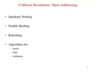
Hash Tables (Cont’d) • Collision resolution strategies • Open addressing (probe table for open slot) • linear, quadratic probing • double hashing • Separate chaining (map to slot that can hold multiple values • In this case slot is called bucket • Approach taken by STL
Graphical Overview Table size = m is prime to help distribute keys evenly
Open Addressing • 2 Steps to Compute Slot • i = hf (key) • Slot = i % m Open Addressing: Each slot holds just 1 key
Collision Resolution with Separate Chaining const size_t TABLE_SIZE = 11; // Prime vector <list<int> > table (TABLE_SIZE); index = hf (key) % TABLE_SIZE; table[index].push_back (key);
Coding Hash Functions // Code hash fn. as function object in C++ // Stateful and easier to use than function pointer struct HashString { size_t operator () (const string& key) const { size_t n = 5381; // Prime size_t i; for (i = 0; i < key.length (); ++i) n = (n * 33 ) + key[i]; // Horner return n; } };
Efficiency of Hashing Methods • Load factor = n / m = # elems / table size • Chaining • represents avg. list length • Avg. probes for successful search ≈ 1 + /2 • Avg. probes for unsuccessful search = • Avg. find, insert, erase: O(1) • Worst case O(1) for ? • Open Addressing • represents ? • If > 0.5, double table size and rehash all elements to new table
Quadratic probing • f(i) = i2 or f(i) = ±i2 • If the table size is prime, a new element can always be inserted if the table is at least half empty
Rehashing • If the table gets too full, operations begin to bog down • Solution: build a new table twice the size (at least – keep prime) and hash all values from the old table into the new table
Problems w/ BSTs • Can degenerate completely to lists • Can become skewed • Most ops are O(d) • Want d to be close to lg(N) • How to correct skewness?
Two BSTs: Same Keys • Insertion sequence: 5, 15, 20, 3, 9, 7, 12, 17, 6, 75, 100, 18, 25, 35, 40 (N = 15)
Notions of Balance • For any node N, depth (N->left) and depth (N->right) differ by at most 1 • AVL Trees • All leaves exist at same level (perfectly balanced!) • 2-3-4 Trees • Number of black nodes on any path from root to leaf is same (black height of tree) • Red-black Trees
2-3-4 Trees • 3 node types • 2-node: 2 children, 1 key • 3-node: 3 children, 2 keys • 4-node: 4 children, 3 keys • All leaves at same level • Logarithmic find, insert, erase
2-3-4 Tree How to Search? Space for 4-Node?
Insert for a 2-3-4 Tree • Top-down • Split 4-nodes as you search for insertion point • Ensures node splits don’t keep propagating upwards • Key operation is split of 4-node • Becomes three 2-nodes • Median key is hoisted up and added to parent node
B A B C A C S T V U S T U V Splitting a 4-Node
Insertion into 2-3-4 Tree • Insertion Sequence: 2, 15, 12, 4, 8, 10, 25, 35, 55, 11, 9, 5, 7 Insert 4 Insert 8
Insertion (Cont’d) Insert 10 Insert 55
12 12 4 4 25 25 2 15 8 10 35 55 8 10 11 15 35 55 2 Split 4-node (4, 12, 25) Insert 11 Insertion (Cont’d) Insert 11 Insert 9
Insertion into 2-3-4 Tree (cont’d) Insert 7
Red-Black Trees • Can represent 2-3-4 tree as binary tree • Use 2 colors • Red indicates node is “bound” to parent • Red node cannot have red child • Preserves logarithmic find, insert, erase • More efficient in time and space
Red-Black Tree Ops • Find? – easy • Insertions • Insert as red node • Require splitting of “4-node” (top-down insertion) • Use color-flip for split (4 cases) • Requires rotations • Deletions • Hard • Several cases – color fix-ups • Remember: RB Trees guarantee lg(N) find’s, insert’s, and erase’s
Four Cases in Splitting of a 4-Node Case 1 Case 2 Case 3 Case 4
Prior to inserting key 55 Case 2
Oriented left-left from G Using A Single Right Rotation P rotated right Case 3 (and G, P, X linear (zig-zig)
Oriented Left-Right From G After the Color Flip Case 4 (and G, P, X zig-zag)
After X is Double Rotated (X is rotated left-right) X P G A B C D
Building A Red-Black Tree right-left rotate