Download
1 / 49
490 likes | 623 Views
Fiber Optics Design and Solving Symmetric Banded Systems. Linda Kaufman William Paterson University. High Speed Optical Communication Segment. EDFA. Dispersion Compensation. Amplification. Transmission (~80km). Dispersion Compensation fibers. Signal degradation and Restoration.

E N D
Fiber Optics Design and Solving Symmetric Banded Systems Linda Kaufman William Paterson University
High Speed Optical Communication Segment EDFA Dispersion Compensation Amplification Transmission (~80km) Dispersion Compensation fibers Signal degradation and Restoration
Fiber Optics Design and Solving symmetric Banded systems Linda Kaufman William Paterson University
Output Input Fiber Optimizer Optimization routine SNOPT Fiber design that achieves transmission target Desired transmission properties * + Objective function formulation * Fiber simulator Manufacturing Constraints Fiber Design
Model-Maxwell’s equation in cylindrical coordinates • For a radially symmetric fiber r is the radius from the center of the fiber, m and ω are known and β and x are unknown. We have a pde-eigenvalue problem. Want to find the relative index profile η such that the dispersion has particular values for specific values of where ω Note η gives the width and dopant concentration of the layers of the fiber and is usually defined by about 20 parameters
1.40 DS1 a 1 0.90 a 4 BD DE4 BE a Index Profile DS4 5 0.40 DE5 DE1 W4 BR W1 a 2 DS5 W5 DE2 -0.10 W3 W6 DS6 DE3 DS2 W1 a 3 DS3 -0.60 0.0 5.0 10.0 15.0 Typical refractive profile and parameterization
Discretization Leads to a nonlinear eigenvalue problem of the form The function s() takes into consideration the boundary condition. If wrapped around a spool Marcuse model leads to 7 diagonal problem
Each function evaluation of an optimizer to determine the parameters of ηrequires • For several values of m • For about 20 values of ω • Determine the grid and make A and M • Solve the nonlinear eigenvalue problem for the positive eigenvalues • Might involve several solutions of a linear eigenvalue problem • Determine the dispersion, dispersion slope and the effective index- an integral of the eigenvectors. The dispersion is given as where ωλ=2πc, c is the speed of light
Difficulties • Numerical difficulties means that numerical differentiation does not work and must supply the gradient of the dispersion- yikes third derivatives! • The eigenvalue problem is slightly nonlinear and gives real problems when β is near zero • Need accurate model so the dispersion has to be computed analytically- means differentiating an eigenvalue • Want to move onto a fiber wrapped around a spool which leads to 7 diagonal problem and solving a symmetric system-where the outermost diagonal has the larger elements and for about 2000 eigenvalues 20 are positive.
Definitions: symmetric,indefinite, banded An n x n matrix A is symmetric if ajk = akj A matrix is indefinite if any of these hold a. eigenvalues are not necessarily all positive or all negative b. One cannot factor A into LLT A has band width 2m+1 if ajk = 0 for |k-j| >m m=2 x x x x x x x 0 x x x x x x x x x x x x x x x 0 x x x x x x x
Applications • Finding intermediate eigenvalues of a symmetric problem that comes from a partial differential equation on a regular grid • Optical fiber design of a fiber wrapped around a spool using Marcuse model • Designing cavity of a linear accelerator • Shift and invert Lanczos • KKT equations-minimizing 1/2xtPx + xtq such that Ax =b gives the optimality conditions
Uses • (1)Solve a system of equations Ax=b If A = MDMT , D is block diagonal, one solves Mz=b Dy =z MTx =y (2)Find the inertia of a system- the number of positive and negative eigenvalues of a matrix If A = MDMT, The inertia of A is the inertia of D. Given a matrix B, the inertia of a matrix A = B-cI is the number of eigenvalues greater, less than and equal to c.
Competition • Ignore symmetry- use Gaussian elimination- does not give inertia info- 0(nm2) time • Band reduction to tridiagonal (Schwarz,Bischof, Lang, Sun, Kaufman) followed by Bunch for tridiagonal-0(n2m) • Snap Back-Irony and Toledo-Cerfacs-2004, 0(nm2) time generally faster than GE but twice space • Bunch – Kaufman for general matrices and hope bandwidth does not grow as Jones and Patrick noticed
Difficulties Consider the linear system .0001x + y = 1.0 x + y = 2.0 Gaussian elimination- 3 digit arithmetic .0001x + y = 1.0 10000y = 10000 Giving y = 1, x =0 But true solution is about x =1.001y =.999 If interchange first and second rows and columns before Gaussian elimination get x + y = 2.0 y = 2.0 -1.0= 1.0 So x = 1.0- a bit better
Gaussian elimination with partial pivoting to prevent division by zero and unbounded elemental growth 1 1 10 1 8 4 6 10 4 3 5 8 6 5 7 1 3 8 1 6 2 1 3 2 5 4 1 4 7 Unsymmetric pivoting yields 10 4 3 5 8 1 8 4 6 1 1 10 6 5 7 1 3 8 1 6 2 1 3 2 5 4 1 4 7 10 4 3 5 8 0 x x x f 0 x x f f 6 5 7 1 3 8 1 6 2 1 3 2 5 4 1 4 7 Eliminating first column yields 5 diagonal becomes 7 diagonal In general 2k+1 diagonal becomes 3k+1 diagonal
Symmetric pivoting • But to maintain symmetry one must pivot rows and columns simultaneously What if matrix is 0 1 ? 1 0 Interchanging first row and column does not help If matrix is 0 1 1000 1 0 10 1000 10 0 Pivot it to 0 1000 1 1000 0 10 1 10 0 And use top 2 x 2 as a “pivot” But pivoting tends to upset the band structure!!
Bunch -Kaufman for symmetric indefinite non banded Where D is either 1 x 1 or 2 x 2 and B’ = B – Y D-1 YT Choice of dimension of D depends on magnitude of a11 versus other elements If D is 2 x 2, det(D)<0 Partition A as
4 2 1 1 0 0 2 3 3 1 x 1 0 2 2.5 1 3 5 0 2.5 4.75 1 10 5 1 0 0 10 200 3 1 x 1 0 100 -47 5 3 8 0 -47 -17 1 10 5 1 10 0 10 50 3 2 x 2 10 50 0 5 3 8 0 0 25.3 2 x 2 vs 1 x 1 for nonbanded symmetric system
1) Let c = |ar 1 | = max in abs. in col. 1 2) If |a11 | >= w c, use a 1 x 1 pivot. Here w is a scalar to balance element growth, like 1/3 Else 3)Let f= max element in abs. in column r 4) If w c*c <= |a11 | f, use a 1 x 1 pivot Else 5)interchange the rth and second rows and columns of A 6) perform a 2 by 2 pivot 7) fix it up if elements stick out beyond the original band width Never pivot with 1 x 1 Banded algorithm based on B-K
Fix up algorithm Worst case r =m+1, what happens in pivoting x x x x x x x x x x x x x a b c d x x x x x x x x x x x x x x x x x x x x x x x x x x x x x x x x x x x x x x x x x x x x x a x x x x x x x x x x b x x x x x x x x x x c x x x x x x x x x d x x x x x x x x x x x x x x x x x x x x x x x x x x x x x
Partition A as • Reset B’ = B – Y D-1 YT • Let Z = D-1 YT = x x x x x x x x x • p q r s x x x x x . • Then B’ looks like • x x x x x x bp cp dp • x x x x x x x cq dq • x x x x x x x cr dr • x x x x x as bs cs ds x • x x x x x x x x x x x x • x x x as x x x x x x x x • bp x x bs x x x x x x x x • cp cq x cs x x x x x x x x • dp dq dr ds x x x x x x x x • x x x x x x x x • x x x x x x x • x x x x x x • If we don’t remove elements outside the band, • the bandwidth could explode to the full matrix.
Because of structure eliminating 1 element gets rid of column x x x x x x x x x x x x x cq dq x x x x x x x cr dr x x x x x x bt ct dt x x x x x x x x x x x x x x x x x x x x x x x x bt x x x x x x x x cq cr ct x x x x x x x x dq dr dt x x x x x x x x x x x x x x x x x x x x x x x x x x x x x
Continue with eliminating another element x x x x x x x x x x x x x x x x x x x x x u x x x x x x x x m x x x x x x x x x x x x x x x x x x x x x x x x x x x x x x x x x x x x x x x x x x x u m x x x x x x x x x x x x x x x x x x x x x x x x x x x x x Now eliminate u to restore bandwidth
In practice one would just use the elements in the first part of Z to determine the Givens/stabilized elementary transformations and never bother to actually form the bulge. Thus there is never any need to generate the elements outside the original bandwidth.
Alternative Formulation Partition A as Where D is 2 x 2 Let Z = D-1 YT Reset B’ = QT(B – Y Z)Q= QTB Q-HG Where H=QTY and G =ZQ Therefore do “retraction” followed by rank 2 correction. Recall H looks like h1 h2 0 h3 Where the “0” has length r-1 and the whole H has length m+r-1
Alternative-2 Q is created such that G =ZQ has the form G = where 0 has r-3 elements and G5 is a multiple of G3 1)Explicitly use 0’s in rank-2 correction Thus correction has form below where numbers indicate the rank of the correction 1 1 0 (r-3 rows) 1 2 1 (m-r+2 rows) 0 1 1 (r-1 rows) 2) Store Q info in place of 0’s and G3 to reduce space to (2m+1)n 3) Reduce solve time for each 2 x 2 from 4m+6r mults to 4m+2r- In worst case, 3mn vs. 5mn
Properties • Space- (2m+1)n-in order to save transformations compared to (3m+1)n for unsymmetric G.E. • Never pivots for positive definite or 1 x 1 • Decrease operations by not applying second column of pivot when these will be undone • Operation count depends on types of transformations • Elementary –between m2n/2 and 5 m2n/4 • Compared with between m2n and 2m2n for G.E.
Elemental growth • Let a = max element of matrix • For 1 x 1, Ajk = Ajk – A1k Aj1 /A11 taking norms element growth is a(1+1/w) • For 2 x 2 if no retraction, it turns out that element growth after 1 step is a(1 + (3+w)/(1-w)) • For 2 x 2 if retraction, it turns out that element growth is (4+8/(1-w))a • 2 steps of 1 x 1 = 1 step of retraction when w=1/3, giving growth bound of 4n-1
Future • Could do pivoting with 1 by 1 at price of space and time- needs to be implemented • Compare time/ element growth with Givens and stabilized elementary • Comparison with Toledo/Irony code and Lapack on bigger machines • Adaptations for small bandwidth as in optical fiber code.
The Nonlinear eigenvalue problem • First attempt Very slow when eigenvalues near 0.
Solve the linear eigenvalue problem using safeguarded Rayleigh quotient
Try to minimize Second attempt: Nonlinear Rayleigh quotient Solution is at
Third Attempt: Newton Approach Find root of Iterate: Where x is an eigenvector of
Easy Problem z=.5
Hard Problem • z=.081
Dispersion When computing A , must also construct A’ and A’’, but these are diagonal. For optimizer really need the derivatives of the dispersion with respect to the design parameters- another layer of differentiation
Dispersion gradient (17) k indicates which of the parameters and there can be about 20
Experimental results 5 positive eigenvalues, 15 design parameters of widths of layers and concentrations, 600 grid points