Download
1 / 21
250 likes | 312 Views
Understand the complexity of combining multiple maps for land analysis, incorporating biophysical factors and social values for effective decision-making. Learn criteria mapping and site ranking techniques in GIS. Explore the potential of ModelBuilder for automating analyses and experimenting with parameters.

E N D
Suitability Analysis in Raster GIS Combining Multiple Maps
The Challenge • Thus far • Single or Dual Factor Overlay Analyses • i.e. Land Cover on Private Land • Biophysical Analyses with Algebraic Formulas • i.e. RUSLE • Landscape Planning • Dozens to hundreds of spatial factors • Factors have “apples and oranges” characteristics • Combinations must reflect social values, not just (bio)physical processes • “Best” for industrial development – from whose perspective? • Therefore • “Suitability Analysis” is not objective - must typically be vetted by experts • If experts are not GIS experts (i.e. local stakeholders), suitability factors and their combination must be visually explained • “Weighting and rating” is a key opportunity for public deliberation
Suitability Analysis • General purpose • To rank potential sites according to suitability for a proposed type of activity • Requirements • A set of “factor” or criteria maps, organized to rate sites relative to one or more characteristics • A technique for appropriately combining factors
Types of Criteria • Absolute • Frequently hard-edged • Often include property ownership/management zones • Often involve legal standards • Relative • Typically “fuzzy” edged • E.g. “proximity to X” where closer = better, but no absolute distance known in advance • Often involved in trade-offs where values ranges come from specific data within a place • Criterion 1 = “Low rent” and criterion 2 = “close to school”
Suitable For Whom? • Suitability models have a “point of view” • Audience can be human • “Affordable housing” • Best sites for High-end commercial • Audience can be environmental • Best habitat for black bear • Most suitable multispecies conservation areas • Can be implicit or explicit • But better to be explicit where possible
Common Units • How do you “combine” • a map representing “meters to nearest road” • Units = meters • with another representing “land cost”? • Units = dollars • Short Answer: find or create common units • Easiest: likert scale “preference” units • A range of values: 1 to 5, or 1 to 9 • Polar opposites on both sides of range • i.e. “Best”/”Worst”, “Most Suitable”/”Completely Unsuitable”
Cautions with Likert Scales • Consistent Application • With multiple factors, must make sure that scale consistently applied • example analysis: want to be near streams and far from roads, using 1..9 with 9 = best • Calculate distance to streams, distance to roads • Reclassify stream distance to preference units • Closest = 0 distance = 9 • Reclassify road distance to preference units • Closest = 0 distance = 1 • In other words, may need to “flip” values when reclassifying • Doesn’t really avoid scaling issues, just defers • Sensitivity and range in price/distance may be different • Often what’s needed from initial analysis is “range of the possible”
Overview • Why Use ModelBuilder? • ModelBuilder Basics • Common ModelBuilder Problems • Advanced ModelBuilder
Why Use ModelBuilder? • An automation tool… • But comes with some startup overhead • Most useful in two circumstances • Documents models & their parameterization • Allows experimentation with model parameters – particularly for “weighting and rating” • Common Types of Models • ETL – Extract, transform and convert raw data • Suitability – Building attractiveness maps
ModelBuilder Basics • Basic idea is that of a “dependency diagram” • User specifies inputs, processing and outputs • If inputs change, system repeats intermediate operations as needed • Diagram has three kinds of elements • Inputs • Geoprocessing Operations • Outputs • Output from one operation can be used as input to an other, allowing “chaining”
ModelBuilder Setup • Rather obscure to start…implemented as a custom toolbox tool • Open toolbox panel • Create empty toolbox • Right mouse on Toolboxes, select New Toolbox • Create empty model • Right mouse on new Toolbox, select New Model • Then populate model by drag and drop • Of data layers from map table of contents • Of geoprocessing operations from the toolbox • Finally, wire data and processing boxes together
Example: Simple MB Model • Goal • Create a factor map expressing simple proximity to residential landuse where output is classed from 1..9 • Method • Create new model • Select residential landuse from San Miguel Parcels database • Add Euclidean distance geoprocessing operation • Connect landuse (input) to distance (process), specifying new grid (output) • Run • Add Reclass Operator • Connect output grid of distance operator to input of reclass, specifying new output grid • Run again
Review of Simple Model • Benefits • Multiple logical steps encapsulated in a single step • Model Logic Recorded in Diagram • Model Parameters Recorded • Problems / Caveats • Default is not to show results… • Model as Created is 100% specific to particular data paths/locations on disk • Model Saving Bizarre.. • Default operation names make no sense to end users • Spatial Analyst Toolbar Options do *not* inherit
Showing Results • Simple, but not Obvious • Right Mouse on Output -> Add to Display • If at first you don’t succeed, try toggling again
Saving / Finding Models • By default, models saved in “My Toolboxes” folder • Main menu Tools->Options->My Toolboxes • Default is C:\Documents and Settings\(Username) \Application Data\ESRI\ArcToolbox\My Toolboxes • Easiest to find in ArcCatalog/My Toolboxes • Can “Add Toolbox” stored on disk
Making Models Generalizable • Running Models • Can Double Click on Models in Toolbox Panel • By default, not too useful, because no user control of outputs • Generalizing Models • By default, models only use exact data originally specified • To make a model into a true “tool” need to specify which inputs / outputs are variable parameters • Right mouse on input or output • Select “Parameter” (toggle) • After Parameters are set, double clicking brings up user dialog
Making MB Diagrams Legible • All elements can be “renamed” from right mouse menu • Rename layers if necessary to clarify • Explain intent of geoprocessing operations • i.e. Isolate Residential Landuse instead of reclass1 • If Desired, change diagram properties • Square – Circle – Square • Box Background Colors • If you need better quality, export diagram…
Environment Variables in MB • Note • Spatial Analyst “Options” settings not inherited • Must explicitly specify for MB • Two options • Can do once for all toolboxes (recommended) • RM Top Toolbox->Environment Settings • General Settings -> Extent • Raster Analysis Settings -> Cell Size • Can do once for each model
Model 2: Weighted Overlay • Goal: • To Create an Attractiveness Model with ability to “Weight” factors • Method: • Create separate ModelBuilder models for each factor • Nest models into master MB model • Combine with weighted overlay
Model 2 Implementation • Factor 1: Proximity to Residential • Factor 2: Proximity to Ski Slopes • Created by copying and pasting factor 1 model and adjusting inputs and outputs • Weighting • Factor 1 = 2X Factor 2 • Use Spatial Analyst Weighted Overlay tool