Download
1 / 15
160 likes | 171 Views
16: Case-Control Odds Ratios. Case-control studies get around several limitations of cohort studies. Relative risks from cohort studies. Use incidences to assess risk Exposed group incidence 1 Non-exposed group incidence 2 RR = ratio of incidence relative measure of effect

E N D
16: Case-Control Odds Ratios Case-control studies get around several limitations of cohort studies Case-Control Odds Ratios
Relative risks from cohort studies • Use incidences to assess risk • Exposed group incidence1 • Non-exposed group incidence2 • RR = ratio of incidence relative measure of effect • Hindrances in Cohort Studies • Long induction period between exposure & disease • Study of rare diseases require large sample sizes • When studying many people information is limited in scope & accuracy Case-Control Odds Ratios
Case-control sample • Study all cases (Proportion exposed reflects exposure proportion of cases in the population) • Select random sample of non-cases (Proportion exposed reflects exposure proportion of non-cases in the population) • This design forfeits the ability to estimate incidence, but maintains ability to estimate relative risk via the odds ratio (Cornfield, 1951; Miettinen 1976) Case-Control Odds Ratios
Illustrative Example (Breslow & Day, 1980) • Dataset = bd1.sav • Exposure variable (alc2) = Alcohol use dichotomized • Disease variable (case) = Esophageal cancer Case-Control Odds Ratios
Interpretation of Odds Ratio • Odds ratios are relative risk estimates • Risk multiplier • e.g., odds ratio of 5.64 suggests 5.64× risk with exposure • Percent increase or decrease in risk (in relative terms) = (odds ratio – 1) × 100% • e.g., odds ratio of 5.64 • Percent relative risk difference = (5.64 – 1) × 100% = 464% Case-Control Odds Ratios
95% Confidence Interval • Calculation • Convert OR estimate to ln scale • SElnOR = sqrt(a-1 + b-1 + c-1 + d-1) • 95% CI for lnOR = (ln OR^) ± (1.96)(SE) • Take anti-logs of limits • Illustrative example • ln(OR^) = ln(5.640) = 1.730 • SElnOR = sqrt(96-1 + 104-1 + 109-1 + 666-1) = 0.1752 • 95% CI for lnOR= 1.730 ± (1.96)(0.1752) = (1.387, 2.073) • 95% CI for OR = e(1.387, 2.073) = (4.00, 7.95) • Interpretation of confidence interval (discuss) Case-Control Odds Ratios
SPSS Output Odds ratio point estimate and confidence limits Ignore “For cohort” information when data derived by case-control sample Case-Control Odds Ratios
Testing H0: OR = 1 with the CI • 95% CI corresponds to a = 0.05 • If 95% CI for odds ratio excludes 1 odds ratio is significant • e.g., (95% CI: 4.00, 7.95) is a significant positive association • e.g., (95% CI: 0.25, 0.65) is a significant negative association • If 95% CI includes 1 odds ratio NOT significant • e.g., (95% CI: 0.80, 1.15) is not significant (i.e., cannot rule out odds ratio parameter of 1 with 95% confidence Also use a chi-square test or Fisher’s test as needed Case-Control Odds Ratios
Chi-Square, Pearson (Do not review) c2Pearson's = (96 - 42.051)2 / 42.051 + (109 – 162.949)2 / 162.949 + (104 - 157.949)2 / 157.949 + (666 – 612.051)2 / 612.051 = 69.213 + 17.861 + 18.427 + 4.755 = 110.256 c = sqrt(110.256) = 10.50 off chart (way into tail) P < .0001 Case-Control Odds Ratios
Chi-Square, Yates (Do not review) c2Pearson's = (|96 - 42.051| - ½)2 / 42.051 + (|109 – 162.949| - ½)2 / 162.949 + (|104 - 157.949| - ½)2 / 157.949 + (|666 – 612.051| - ½)2 / 612.051 = 67.935 + 17.532 + 18.087 + 4.668 = 108.221 c = sqrt(108.22) = 10.40 P < .0001 Case-Control Odds Ratios
SPSS Output Pearson = uncorrected Yates = continuity corrected Fisher’s unnecessary here Linear-by-linear not covered Case-Control Odds Ratios
Matched-Pairs Matching can be employed to help control for confounding (e.g., matching on age and sex), with each pair representing an observation. Calculate 95% CI for ln OR with (ln estimate) ± (1.96)(SE) and then take anti-logs of limits Case-Control Odds Ratios
Example (Matched Pairs) Case-Control Odds Ratios
Validity Conditions! • No info bias (data accurate) • No selection bias (cases and controls random reflection of population analogues) • No confounding (association not explained by lurking factors!) Validity conditions are nearly always the limiting factor in practice. Case-Control Odds Ratios
McNemar’s Test for Matched Pairs (not covered, use CI instead) Use McNemar’s chi-square to test H0: OR = 1 (“no association”) for binary matched paired P for current example = 0.0016 Case-Control Odds Ratios

![16: Odds Ratios [from case-control studies]](https://cdn0.slideserve.com/464336/16-odds-ratios-from-case-control-studies-dt.jpg)