Download
1 / 17
170 likes | 672 Views
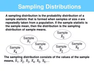
Sampling distributions . The sampling distribution of the mean The Central Limit Theorem The Normal Deviate Test (Z for samples). Sampling distributions. The distribution of a statistic (eg. mean, median, standard deviation) for the set of all possible samples from a population.

E N D
Sampling distributions The sampling distribution of the mean The Central Limit Theorem The Normal Deviate Test (Z for samples)
Sampling distributions • The distribution of a statistic (eg. mean, median, standard deviation) for the set of all possible samples from a population. • For example, if we toss an unbiased coin repeatedly in sets of three tosses, scoring heads as 1 and tails as 0, the possible samples are as follows:
An example SampleMean HHH 1.00 HHT .67 HTH .67 THH .67 TTH .33 THT .33 HTT .33 TTT .00 Sampling Distribution of the mean Meanf 1.00 1 .67 3 .33 3 .00 1 8 p .125 .375 .375 .125 1.00
Characteristics of the sampling distribution • It includes all of the possible values of a statistic for samples of a particular n • It includes the frequency or probability of each value of a statistic for samples of a particular n
Another example • Imaginary marbles • Invisible vessels: n = 100 • Marking means: Poker chips • In the kitty: The sampling distribution of the mean.
The null hypothesis population • The entire set of scores as they are naturally, that is, if the treatment has not affected them. • If the treatment has had no effect, then the null hypothesis is true: thus, the name null hypothesis population. • If a treatment has an effect, then the mean of the treated sample will not fit well in the null hypothesis population: It will be weird.
The Central Limit Theorem • If random samples of the same size are drawn from any population, then • the mean of the sampling distribution of the mean approaches m , and • the standard deviation of the sampling distribution, called the standard error of the mean, approaches s / n ... • as n gets larger.
Generating a sampling distribution • From a population of six people who are given grape Kool-Aid, persons 1, 2, and 3 have their IQs raised, and persons 4, 5, and 6 have their IQs go down. • Sampling without replacement, form all of the possible unique samples of 2 people from the population of six. (Simplified example) • In how may of the samples does the mean IQ increase?
The normal deviate test • The normal deviate test is the Z test applied to sample means. • To use it, you must know the population mean and standard deviation. You may know these as • Population measurements • TQM or CQI goals • Design parameters • Historical sample patterns
The normal deviate test... • The only difference from the simple Z test is that the denominator is s / n , which is known as the standard error of the mean. • To test our grape Kool-Aid gang, take a sample of 100 Houghton students, and compute the mean IQ = 130. Compare that mean to a population mean of 125, with a population standard deviation of 15.
The critical region • You can simplify a set of decisions about sample means by establishing the critical region for sample means which fit a rejection criterion for Z. • For a one-tailed test at the .05 level, the critical value of Z from table B-1 is 1.645 • For a two-tailed test at the .05 level, the critical value of Z is 1.96
Calculating the critical region • Plug the appropriate critical value of Z (1.645 or 1.96) into the equation for the normal deviate test, and solve for M. • Remember that for a two-tailed test, the critical sample mean for each tail must be calculated by working above and below the population mean m.
Sample size and power • Test the grape Kool-aid gang again, with sample sizes of 4, 9, 16, 25, 36, 49, 64, and 81. • You will notice that as the sample size increases, the obtained Z-score for the same size difference between means also increases. • If the same difference produces a larger Z-score, the test has more power.
When can we use the normal deviate Z-test? • For a single sample mean • When we know m and s • When the sampling distribution of the mean is normally distributed, which we can usually assume when n is 30 or more • Notable exception: reaction time measures
Reporting standard error in APA format • In text or in tables, report standard error with the abreviation SE. • In graphs, indicate the size of the standard error with error bars, bracketed lines centered at the top of the bar of the graph for the mean, and extending one standard error above and below the mean.
Normal deviate test in APA • z = 1.98, p < .05 • z = 1.95, p > .05 • z = 1.40, p = .08