Download
1 / 27
270 likes | 392 Views
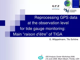
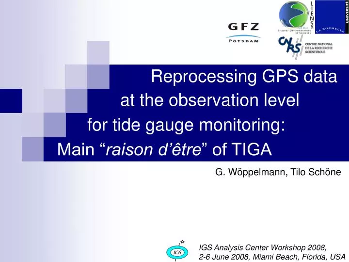
Reprocessing GPS data. at the observation level. for tide gauge monitoring:. Main “ raison d’être ” of TIGA. G. Wöppelmann, Tilo Schöne. IGS Analysis Center Workshop 2008, 2-6 June 2008, Miami Beach, Florida, USA. Overview. I. What are the sea-level applications requirements?

E N D
Reprocessing GPS data at the observation level for tide gauge monitoring: Main “raison d’être” of TIGA G. Wöppelmann, Tilo Schöne IGS Analysis Center Workshop 2008, 2-6 June 2008, Miami Beach, Florida, USA
Overview I. What are the sea-level applications requirements? II. The TIGA Pilot Project III. An example: Reprocessing Strategy at ULR IV. Some important issues to do with cGPS@TG V. Outlooks
“Sea-level enigma” (Munk 2002) Sum of climatic contributions to sea level rise: ~0.7mm/yr Analyses of tide gauge records ~1.5mm/yr IPCC (2007) 1.1 mm/yr 1.8 mm/yr I. Long term sea level trends IPCC (2001) WRCP Workshop in 2006 Reducing uncertainties in past and present sea level rise…
Challenges • Rates in sea-level change: ~1-2 mm/yr • Standard errors several times smaller to be useful in these studies! “Important issues to do with long term sea level trends” (e.g. Woodworth 2006, in Phil. Trans. R. Soc.) • Vertical land motion at tide gauges • Stockholm : Post-glacial rebound • Nezugaseki : 1964 earthquake • Bangkok : Ground water pumping • Manila : Sedimentation (Glacial isostatic adjustment) (Co-seismic displacement) (Groundwater extraction) • Motivation for GPS reprocessing • To use the best available data and most accurate models to reduce errors in the estimates of coordinates • To use them all over the data span (models, parameterization…) in order to derive consistent sets of station coordinates, and to limit spurious signals in their time series (Sedimentation) (No evidence of land motion)
I… Radar altimetry calibration • Altimetric data • 4 closest passes to the tide gauge (Ǿ<160km) • Closest points to the tide gauges over each pass, with valid SLA content: 70% of valid values w.r.t. the total # of cycles • Tide gauge data • Time series > 2 years • Interpolation at the epoch of altimetric pass • Data editing (Mitchum 2000) • Minimum correlation: 0.3 (SLA Alt / TG) • Maximum RMS differnces: 100mm
GFT ULR ETG DGF AUT CTA II. The TIGA pilot project (Initiated in 2001, on a best-effort basis) http://adsc.gfz-potsdam.de/tiga/index_TIGA.html • “Tide Gauge Benchmark Monitoring” • 103 TOS, 2 TDC, 6 TAC, TAAC (?) • Goals • Establish, maintain and expand a global cGPS@TG network • Compute precise station parameters for the cGPS@TG stations with a high latency • Reprocess all previously collected GPS data, if possible back to 1993 • Promote the establishment of links to other geodetic sites (DORIS, SLR, VLBI,… AG)
III. An example: ULR Analysis Centre • Total # of GPS stations: 225 • IGS05 stations: 91 • Time span: 1997.0 - 2006.9 • 205 time series > 3.5 years • 160 are co-located with TG • 90 CGPS@TG are not IGS
III… Reprocessing analysis strategy at ULR Stacking of the weekly station coordinate solutions using Altamimi et al. (2002, 2007) approach published in JGR. OUTPUTS station positions and velocities at t0 (2001/346), as well as, time series of post-fit residuals (station coordinates), time series of transformation parameters, between each weekly solution and the final stacked one discontinuities estimates (iterative procedure to detect outliers and discontinuities)
III… GPS velocities at TG... How well do they work? ICE5Gv1.2 + VM4 models (Peltier 2004) For details: Wöppelmann et al. Poster to be displayed Thursday… also, paper published in Global and Planetary Change (2007)
ITRF2000 1999.0-2005.7 6.7 years Table1 from Wöppelmann et al. 2007 (Glob. Planet. Change) 1.56 ± 2.05 1.28 ± 1.34 1.69 ± 1.49
Newuncertainties Updated from our recent GPS re-analysis 1.28 ± 1.34 1.69 ± 1.49 1.37 ± 1.25 1.68 ± 1.15
IV. Some important issues to do with cGPS@TG • Working hypotheses 1. Land movements are linear over the tide gauge records length 2. GPS antenna vertical movement Tide gauge land movement • Some examples… • Local land motion monitoring (stability) • geodetic link between GPS antenna and TGBM • ancillary local information (equipment changes, topography…) specially, if the GPS was not installed for sea level studies! Leadership issue raised at EGU 2008, Vienna.
VERTICAL -0.640.01 -0.750.01 IV… Assessing the quality of the GPS results Stacked periodograms for filtered GPS position time series • 75 GPS stations in common with > 200 weekly points over the 1997.0-2006.0 period • Lomb-Scargle periodogram (Press et al. 2001) • Normalized spectra stacked and filtered following Ray et al. (2008) approach (annual and semi-annual fits have been removed prior to spectra computation)
EAST -0.480.01 -0.710.01 IV… Assessing the quality of our GPS results Stacked periodograms for filtered GPS position time series • 75 GPS stations in common with > 200 weekly points over the 1997.0-2006.0 period • Lomb-Scargle periodogram (Press et al. 2001) • Normalized spectra stacked and filtered following Ray et al. (2008) approach (annual and semi-annual fits have been removed prior to spectra computation)
NORTH -0.580.01 -0.700.01 IV… Assessing the quality of our GPS results Stacked periodograms for filtered GPS position time series Detection of anomalous harmonics… (Ray et al. 2008)
it00 it05 IV. Some important issues to do with cGPS@TG Summary of the long-term sea level trend study Douglas & Peltier (2001): 1.840.35mm/yr ITRF2000 versus ITRF2005 Impact on the vertical velocities… Which reference frame?
IV… ITRF2000 versus ITRF2005 datum Impact on vertical velocities: using ITRF2005 datum or ITRF2000
IV… ITRF2000 versus ITRF2005 datum Transformation parameters estimated from our GPS solutions (ITRF2005 → ITRF2000) ~ 0.83 mm/yr
Shennan & Horton (2002) Inferred from PSMSL (2005) and Holgate & Woodworth (2004) IV… Vertical land motion to be interpreted
V. Conclusions and Outlooks • Promising scientific results • Combined TIGA solution pending (provided soon…). • Reprocessing with absolute PCV ongoing • Volunteers for combination analyses needed • Trying to secure long(er)-term funding for processing and combination So far best-effort basis • Efforts are needed for meta-data information (e.g. leveling between benchmarks and TG zero) Leadership issue… • Need for a more robust and stable ITRF • Current accuracy: 1-2 mm/yr origin, 0.1 ppb/yr scale • Target accuracy: 0.1 mm/yr origin, 0.01 ppb/yr scale
Current (103) and potential (300) cGPS@TG stations • Towards an improved reprocessing (VMF1,…) • Upgrade the reprocessing capabilities (1 year 1 week) • Potential for 300 cGPS@TG • Access to data and meta-data • Clustering in populated areas
Thank you for your attention ! View of La Rochelle
Stacking of weekly GPS solutions in SINEX format Inputs : Weekly solutions (…) X(ts) – SINEX files (Each individual solution defines its own reference frame...) Model : Outputs : Combined solution : positions Xitrf(t0), and velocities Time series of transformation parameters between each individual solution and the combined one (Tx, Ty, Tz, D, Rx, Ry, Rz) Time series of post-fit residuals (station coordinates…) The reference frame is defined by applying minimal constraints Model implemented in CATREF (Altamimi, 2004)
Transformation parameters between each weekly solution and the combined one expressed in ITRF2000 or ITRF2005
Motivation: Compute realistic uncertainties on GPS velocities. Zhang et al. (1997): Noise in GPS position time series • Many geophysical phenomena can be described using a power-law process of the form (Agnew, 1992): : spectral index. = 0 White Noise (WN); =-1 Flicker Noise (FN); =-2, Random Walk Noise (RWN) • Methods: • MLE, Maximum Likelihood Estimation e.g. Williams et al. (2003, 2004,…) • SPECTRAL ANALYSIS e.g. Zhang et al. (1997), Mao et al. (1999) • ALLAN VARIANCE • Stability of atomic clocks, e.g. Allan (1966) • Method adapted to geodetic data, e.g. Le-Bail (2006), Feissel-Vernier et al. (2007)
Other altimetry missions… Without GPS-velocities corrections • Very preliminary results… to be confirmed and further investigated • Comparable drifts for Jason-1, T/P and GFO missions • Drifts between 0.5 - 1.0 mm/yr without land motion correction • Drifts closer to 0 mm/yr with GPS-derived corrections from GPC solution. • Only Envisat still shows a significant drift With GPS-velocities corrections