Download
1 / 31
310 likes | 450 Views
Review of Probability and Statistics. ECON 345 - Gochenour. Random Variables. X is a random variable if it represents a random draw from some population a discrete random variable can take on only selected values a continuous random variable can take on any value in a real interval

E N D
Review of Probability and Statistics ECON 345 - Gochenour
Random Variables • X is a random variable if it represents a random draw from some population • a discrete random variable can take on only selected values • a continuous random variable can take on any value in a real interval • associated with each random variable is a probability distribution
Random Variables – Examples • the outcome of a coin toss – a discrete random variable with P(Heads)=.5 and P(Tails)=.5 • the height of a selected student – a continuous random variable drawn from an approximately normal distribution
Expected Value of X – E(X) • The expected value is really just a probability weighted average of X • E(X) is the mean of the distribution of X, denoted by mx • Let f(xi) be the probability that X=xi, then
Variance of X – Var(X) • The variance of X is a measure of the dispersion of the distribution • Var(X) is the expected value of the squared deviations from the mean, so
More on Variance • The square root of Var(X) is the standard deviation of X • Var(X) can alternatively be written in terms of a weighted sum of squared deviations, because
Covariance – Cov(X,Y) • Covariance between X and Y is a measure of the association between two random variables, X & Y • If positive, then both move up or down together • If negative, then if X is high, Y is low, vice versa
Correlation Between X and Y • Covariance is dependent upon the units of X & Y [Cov(aX,bY)=abCov(X,Y)] • Correlation, Corr(X,Y), scales covariance by the standard deviations of X & Y so that it lies between 1 & –1
More Correlation & Covariance • If sX,Y =0 (or equivalently rX,Y =0) then X and Y are linearly unrelated • If rX,Y = 1 then X and Y are said to be perfectly positively correlated • If rX,Y = – 1 then X and Y are said to be perfectly negatively correlated • Corr(aX,bY) = Corr(X,Y) if ab>0 • Corr(aX,bY) = –Corr(X,Y) if ab<0
Properties of Expectations • E(a)=a, Var(a)=0 • E(mX)=mX, i.e. E(E(X))=E(X) • E(aX+b)=aE(X)+b • E(X+Y)=E(X)+E(Y) • E(X-Y)=E(X)-E(Y) • E(X- mX)=0 or E(X-E(X))=0 • E((aX)2)=a2E(X2)
More Properties • Var(X) = E(X2) – mx2 • Var(aX+b) = a2Var(X) • Var(X+Y) = Var(X) +Var(Y) +2Cov(X,Y) • Var(X-Y) = Var(X) +Var(Y) - 2Cov(X,Y) • Cov(X,Y) = E(XY)-mxmy • If (and only if) X,Y independent, then • Var(X+Y)=Var(X)+Var(Y), E(XY)=E(X)E(Y)
The Normal Distribution • A general normal distribution, with mean m and variance s2 is written as N(m, s2) • It has the following probability density function (pdf)
The Standard Normal • Any random variable can be “standardized” by subtracting the mean, m, and dividing by the standard deviation, s , so E(Z)=0, Var(Z)=1 • Thus, the standard normal, N(0,1), has pdf
Properties of the Normal • If X~N(m,s2), then aX+b ~N(am+b,a2s2) • A linear combination of independent, identically distributed (iid) normal random variables will also be normally distributed • If Y1,Y2, … Yn are iid and ~N(m,s2), then
Cumulative Distribution Function • For a pdf, f(x), where f(x) is P(X = x), the cumulative distribution function (cdf), F(x), is P(X x); P(X > x) = 1 – F(x) =P(X< – x) • For the standard normal, f(z), the cdf is F(z)= P(Z<z), so • P(|Z|>a) = 2P(Z>a) = 2[1-F(a)] • P(a Z b) = F(b) – F(a)
The Chi-Square Distribution • Suppose that Zi , i=1,…,n are iid ~ N(0,1), and X=(Zi2), then • X has a chi-square distribution with n degrees of freedom (df), that is • X~2n • If X~2n, then E(X)=n and Var(X)=2n
The t distribution • If a random variable, T, has a t distribution with n degrees of freedom, then it is denoted as T~tn • E(T)=0 (for n>1) and Var(T)=n/(n-2) (for n>2) • T is a function of Z~N(0,1) and X~2n as follows:
The F Distribution • If a random variable, F, has an F distribution with (k1,k2) df, then it is denoted as F~Fk1,k2 • F is a function of X1~2k1 and X2~2k2 as follows:
Random Samples and Sampling • For a random variable Y, repeated draws from the same population can be labeled as Y1, Y2, . . . , Yn • If every combination of n sample points has an equal chance of being selected, this is a random sample • A random sample is a set of independent, identically distributed (i.i.d) random variables
Estimators and Estimates • Typically, we can’t observe the full population, so we must make inferences base on estimates from a random sample • An estimator is just a mathematical formula for estimating a population parameter from sample data • An estimate is the actual number the formula produces from the sample data
Examples of Estimators • Suppose we want to estimate the population mean • Suppose we use the formula for E(Y), but substitute 1/n for f(yi) as the probability weight since each point has an equal chance of being included in the sample, then • Can calculate the sample average for our sample:
What Make a Good Estimator? • Unbiasedness • Efficiency • Mean Square Error (MSE) • Asymptotic properties (for large samples): • Consistency
Unbiasedness of Estimator • Want your estimator to be right, on average • We say an estimator, W, of a Population Parameter, q, is unbiased if E(W)=E(q) • For our example, that means we want
Efficiency of Estimator • Want your estimator to be closer to the truth, on average, than any other estimator • We say an estimator, W, is efficient if Var(W)< Var(any other estimator) • Note, for our example
MSE of Estimator • What if can’t find an unbiased estimator? • Define mean square error as E[(W-q)2] • Get trade off between unbiasedness and efficiency, since MSE = variance + bias2 • For our example, that means minimizing
Consistency of Estimator • Asymptotic properties, that is, what happens as the sample size goes to infinity? • Want distribution of W to converge to q, i.e. plim(W)=q • For our example, that means we want
More on Consistency • An unbiased estimator is not necessarily consistent – suppose choose Y1 as estimate of mY, since E(Y1)= mY, then plim(Y1) mY • An unbiased estimator, W, is consistent if Var(W) 0 as n • Law of Large Numbers refers to the consistency of sample average as estimator for m, that is, to the fact that:
Central Limit Theorem • Asymptotic Normality implies that P(Z<z)F(z) as n , or P(Z<z) F(z) • The central limit theorem states that the standardized average of any population with mean m and variance s2 is asymptotically ~N(0,1), or
Estimate of Population Variance • We have a good estimate of mY, would like a good estimate of s2Y • Can use the sample variance given below – note division by n-1, not n, since mean is estimated too – if know m can use n
Estimators as Random Variables • Each of our sample statistics (e.g. the sample mean, sample variance, etc.) is a random variable - Why? • Each time we pull a random sample, we’ll get different sample statistics • If we pull lots and lots of samples, we’ll get a distribution of sample statistics