Download

1 / 44
450 likes | 596 Views
Dynamics of bosonic cold atoms in optical lattices. K. Sengupta Indian Association for the Cultivation of Science, Kolkata. Collaborators: Anirban Dutta , Brian Clark, Uma Divakaran , Michael Kobodurez , Shreyoshi Mondal , David Pekker , Rajdeep Sensarma & Christian Trefzger.

E N D
Dynamics of bosonic cold atoms in optical lattices. K. Sengupta Indian Association for the Cultivation of Science, Kolkata Collaborators: AnirbanDutta, Brian Clark, UmaDivakaran, Michael Kobodurez, ShreyoshiMondal, David Pekker, RajdeepSensarma & Christian Trefzger
Overview 1. Introduction to ultracold bosons 2. Dynamics of the Bose-Hubbard model 3. Dynamics induced freezing 4. Bosons in an electric field: Theory and experiments 5. Dynamics of bosons in an electric field 6. Extension to trapped system [work in progress] 7. Conclusion
Cooling atoms: how cold is ultracold Perspective about how cold these atoms really are: coldest place in the universe How do you measure such temperatures? Form a BEC and measure the width of the central peak in its momentum distribution. Hot Cold
Cooling techniques: two methods Doppler cooling of atoms Creation of optical molasses leading to microkelvin temperatures Further evaporative cooling of the atoms leading to temperature ~ 10 nK This is well below critical Temperature of a BEC
Emulating lattices for bosons with light Apply counter propagating laser: standing wave of light. The atoms feel a potential V = -a |E|2 For positive a, the atoms sits at the bottom of the potential generated by the lasers: Bloch theory for bosons
From BEC to the Mott state Apply counter propagating laser: standing wave of light. The atoms feel a potential V = -a |E|2 Energy Scales For a deep enough potential, the atoms are localized : Mott insulator described by single band Bose-Hubbard model. dEn= 5Er ~ 20 U U ~10-300 t Model Hamiltonian Ignore higher bands
Mott-Superfluid transition: preliminary analysis Mott state with 1 boson per site Stable ground state for 0 < m < U Mott state is destabilized when the excitation energy touches 0. Adding a particle to the Mott state Removing a particle from the Mott state Destabilization of the Mott state via addition of particles/hole: onset of superfluidity
Beyond this simple picture Higher order energy calculation by Freericks and Monien: Inclusion of up to O(t3/U3) virtual processes. Mean-field theory (Fisher 89, Seshadri 93) Phase diagram for n=1 and d=3 Quantum Monte Carlo studies for 2D & 3D systems: Trivedi and Krauth, B. Sansone-Capponegro O(t2/U2) theories MFT Superfluid Predicts a quantum phase transition with z=2 (except at the tip of the Mott lobe where z=1). Mott No method for studying dynamics beyond mean-field theory
Distinguishing between hopping processes Mott state Distinguish between two types of hopping processes using a projection operator technique Define a projection operator Divide the hopping to classes (b) and (c)
Building fluctuations over MFT Design a transformation which eliminate hopping processes of class (b) perturbatively in J/U. Obtain the effective Hamiltonian Use the effective Hamiltonian to compute the ground state energy and hence the phase diagram
Equilibrium phase diagram Reproduction of the phase diagram with remarkable accuracy in d=3: much better than standard mean-field or strong coupling expansion in d=2 and 3. Accurate for large z as can be checked by comparing with QMC data for 2D triangular (z=6) and 3D cubic lattice Allows for straightforward generalization for treatment of dynamics
Non-equilibrium dynamics: Linear ramp Consider a linear ramp of J(t)=Ji +(Jf- Ji) t/t. For dynamics, one needs to solve the Sch. Eq. Make a time dependent transformation to address the dynamics by projecting on the instantaneous low-energy sector. The method provides an accurate description of the ramp if J(t)/U <<1 and hence can treat slow and fast ramps at equal footing. Takes care of particle/hole production due to finite ramp rate
F Absence of critical scaling: may be understood as the inability of the system to access the critical (k=0) modes. Fast quench from the Mott to the SF phase; study of superfluid dynamics. Single frequency pattern near the critical Point; more complicated deeper in the SF phase. Strong quantum fluctuations near the QCP; justification of going beyond mft.
Experiments with ultracold bosons on a lattice: finite rate dynamics 2D BEC confined in a trap and in the presence of an optical lattice. Single site imaging done by light-assisted collision which can reliably detect even/odd occupation of a site. In the present experiment they detect sites with n=1. Ramp from the SF side near the QCP to deep inside the Mott phase in a linear ramp with different ramp rates. The no. of sites with odd n displays plateau like behavior and approaches the adiabatic limit when the ramp time is increased asymptotically. No signature of scaling behavior. Interesting spatial patterns. W. Bakr et al. Science 2010
Power law ramp Use a power-law ramp protocol Slope of both F and Q depends on a; however, the plateau-like behavior at large t is independent of a. Absence of Kibble-Zureck scaling for any a due to lack of contribution of small k (critical) modes in the dynamics.
Dynamics induced freezing Tune J from superfluid phase to Mott and back through the tip of the Mott lobe. Key result There are specific frequencies at which the wavefunction of the system comes back to itself after a cycle of the drive leading to P=1-F -> 0. Dynamics induced freezing
Mean-field analysis: A qualitative picture 1. Choose a gutzwillerwavefunction: 2.The mean-field equations for fn En is the on-site energy of the state |n> 3. Numerical solution of this equation indicates that fn vanishes for n>2 for all ranges of drive frequencies studied. 4. Analysis of these equations leads to the relation involving
5. Thus one can describe the system in terms of three real variables : amplitude of state |1> and the sum and difference of the relative phases. fs=f0+f2-2f1fd=f2-f0 6. One can construct a frequency- independent relation between r1 and fs Numerical solution of (6) There is a range of frequency for which r1 and fs remain close to their original values; dynamics induced freezing occurs when fd/4p = n within this range.
Robustness against quantum fluctuations and presence of a trap Mean-field theory Projection operator formalism Density distribution of the bosons inside a trap Robust freezing phenomenon
Applying an electric field to the Mott state Energy Scales: hwn = 5Er »20 U U »10-300 J
Construction of an effective model: 1D Parent Mott state
Charged excitations quasiparticle quasihole
Neutral dipoles Resonantly coupled to the parent Mott state when U=E. Neutral dipole state with energy U-E. Two dipoles which are not nearest neighbors with energy 2(U-E).
Weak Electric Field For weak electric field, the ground state is dipole vaccum and the low-energy excitations are single dipole • The effective Hamiltonian for the dipoles for weak E: • Lowest energy excitations: Single band of dipole excitations. • These excitations soften as E approaches U. This is a precursor of the appearance of Ising density wave with period 2. • Higher excited states consists of multiparticle continuum.
Strong Electric field • The ground state is a state of maximum dipoles. • Because of the constraint of not having two dipoles on consecutive sites, we have two degenerate ground states • The ground state breaks Z2 symmetry. • The first excited state consists of band of domain walls between the two filled dipole states. • Similar to the behavior of Ising model in a transverse field.
Intermediateelectric field: QPT Quantum phase transition at E-U=1.853w. Ising universality.
Recent Experimental observation of Ising order (Bakr et al Nature 2010) First experimental realization of effective Ising model in ultracold atom system
Quench dynamics across the quantum critical point Tune the electric field from Ei to Ef instantaneously Compute the dipole order Parameter as a function of time The time averaged value of the order parameter is maximal near the QCP
Generic critical points: A phase space argument The system enters the impulse region when rate of change of the gap is the same order as the square of the gap. For slow dynamics, the impulse region is a small region near the critical point where scaling works The system thus spends a time T in the impulse region which depends on the quench time In this region, the energy gap scales as Thus the scaling law for the defect density turns out to be Generalization to finite system size finite-size scaling
Dynamics with a finite rate: Kibble-Zureck scaling Change the electric field linearly in time with a finite rate v Theory Quantities of interest Experiment Scaling laws for finite –size systems Q ~ v2 (v) for slow (intermediate) quench. These are termed as LZ(KZ) regimes for finite-size systems.
Kibble-Zureck scaling for finite-sized system Observation of Kibble-Zurek law for intermediate v with Ising exponents. Expected scaling laws for Q and F Dipole dynamics Correlation function
Periodic dynamics: obtaining zero defect density Protocol Choose dE such that one starts from the dipole vacuum at t=0, goes to the maximally ordered state at t=p/w so that E(t) vanishes at t= (n+1/2)p/w The dipole excitation density for an intermediate frequency range vanishes at special points where the instantaneous electric field vanishes E(t)=U i.e. at t= (n+1/2)p/w
Presence of a trap: spatially varying chemical potential The chemical potential increases as we move from the center to the edges of the trap: One gets multiple MI and SF phases as one moves from the center to the edges of the trap. Clearly the projection operator method will fail since at some sites one may have a value of the chemical potential which equally favors both n=1 and n=2 (or 0) occupation. One can not project to a fixed number and hence can not determine the projection operator uniquely.
Hopping expansion technique for bosons Consider two neighboring sites in the trap with boson occupations can take positive or negative integer values i=1(2) for right(left) hopping: these cost different energy due to the trap. The hopping between these two sites costs an energy 3. One can rewrite the hopping term Right hopping Left hopping 4.We identify the value of for which can be both a positive or negative Integer and may not even exist for a given link
Next, one designs a canonical transformation operator S which eliminates all hoppings to linear order which has 6. One then finds the effective low-energy Hamiltonian using Generalization of the projection operator formalism
Quench and Ramp dynamics Protocol: Linear ramp or quench of the hopping amplitude J Schrodinger equation to be solved One can convert this into an Schrodinger equation for the effective low-energy Hamiltonian One can obtain a set of equations for The Gutzwiller coefficient which can be solved numerically Advantage: General method for treatment of non-equilibrium trapped/disordered bosons beyond mean-field theory Weakness: Can not take long-wavelength quantum fluctuations into account.
Quench from superfluid to MI phase: preliminary results The order parmeter oscillations die after reaching a point for which dm r= J or r = Int[J/K-0.5] The time period dimishes linearly With increasing K