Download
1 / 27
270 likes | 314 Views
This chapter covers determining deformation of axially loaded members, finding support reactions, and analyzing thermal stress, stress concentrations, inelastic deformations, and residual stress in engineering structures.

E N D
CHAPTER OBJECTIVES • Determine deformation of axially loaded members • Develop a method to find support reactions when it cannot be determined from equilibrium equations Analyze the effects of thermal stress, stress concentrations, inelastic deformations, and residual stress
CHAPTER OUTLINE • Saint-Venant’s Principle • Elastic Deformation of an Axially Loaded Member • Principle of Superposition • Statically Indeterminate Axially Loaded Member • Force Method of Analysis for Axially Loaded Member • Thermal Stress • Stress Concentrations • *Inelastic Axial Deformation • *Residual Stress
4.1 SAINT-VENANT’S PRINCIPLE • Localized deformation occurs at each end, and the deformations decrease as measurements are taken further away from the ends • At section c-c, stress reaches almost uniform value as compared to a-a, b-b c-c is sufficiently far enough away from P so that localized deformation “vanishes”, i.e., minimum distance
4.1 SAINT-VENANT’S PRINCIPLE • General rule: min. distance is at least equal to largest dimension of loaded x-section. For the bar, the min. distance is equal to width of bar • This behavior discovered by Barré de Saint-Venant in 1855, this the name of the principle • Saint-Venant Principle states that localized effects caused by any load acting on the body, will dissipate/smooth out within regions that are sufficiently removed from location of load • Thus, no need to study stress distributions at that points near application loads or support reactions
4.2 ELASTIC DEFORMATION OF AN AXIALLY LOADED MEMBER • Relative displacement (δ) of one end of bar with respect to other end caused by this loading • Applying Saint-Venant’s Principle, ignore localized deformations at points of concentrated loading and where x-section suddenly changes
P(x) A(x) dδ dx σ = = P(x) A(x) dδ dx ( ) = E P(x) dx A(x) E dδ= 4.2 ELASTIC DEFORMATION OF AN AXIALLY LOADED MEMBER Use method of sections, and draw free-body diagram Assume proportional limit not exceeded, thus apply Hooke’s Law σ = E
P(x) dx A(x) E ∫0 L δ= 4.2 ELASTIC DEFORMATION OF AN AXIALLY LOADED MEMBER Eqn. 4-1 δ = displacement of one pt relative to another pt L = distance between the two points P(x) = internal axial force at the section, located a distance x from one end A(x) = x-sectional area of the bar, expressed as a function of x E = modulus of elasticity for material
PL AE δ= 4.2 ELASTIC DEFORMATION OF AN AXIALLY LOADED MEMBER Constant load and X-sectional area • For constant x-sectional area A, and homogenous material, E is constant • With constant external force P, applied at each end, then internal force P throughout length of bar is constant • Thus, integrating Eqn 4-1 will yield Eqn. 4-2
PL AE δ= 4.2 ELASTIC DEFORMATION OF AN AXIALLY LOADED MEMBER Constant load and X-sectional area • If bar subjected to several different axial forces, or x-sectional area or E is not constant, then the equation can be applied to each segment of the bar and added algebraically to get
4.2 ELASTIC DEFORMATION OF AN AXIALLY LOADED MEMBER Sign convention
4.2 ELASTIC DEFORMATION OF AN AXIALLY LOADED MEMBER Procedure for analysis Internal force • Use method of sections to determine internal axial force P in the member • If the force varies along member’s strength, section made at the arbitrary location x from one end of member and force represented as a function of x, i.e., P(x) • If several constant external forces act on member, internal force in each segment, between two external forces, must then be determined
4.2 ELASTIC DEFORMATION OF AN AXIALLY LOADED MEMBER Procedure for analysis Internal force • For any segment, internal tensile force is positive and internal compressive force is negative. Results of loading can be shown graphically by constructing the normal-force diagram Displacement • When member’s x-sectional area varies along its axis, the area should be expressed as a function of its position x, i.e., A(x)
4.2 ELASTIC DEFORMATION OF AN AXIALLY LOADED MEMBER Procedure for analysis Displacement • If x-sectional area, modulus of elasticity, or internal loading suddenly changes, then Eqn 4-2 should be applied to each segment for which the qty are constant • When substituting data into equations, account for proper sign for P, tensile loadings +ve, compressive −ve. Use consistent set of units. If result is +ve, elongation occurs, −ve means it’s a contraction
EXAMPLE 4.1 Composite A-36 steel bar shown made from two segments AB and BD. Area AAB = 600 mm2and ABD = 1200 mm2. Determine the vertical displacement of end A and displacement of B relative to C.
EXAMPLE 4.1 (SOLN) Internal force Due to external loadings, internal axial forces in regions AB, BC and CD are different. Apply method of sections and equation of vertical force equilibrium as shown. Variation is also plotted.
[+75 kN](1 m)(106) [600 mm2 (210)(103) kN/m2] PL AE δA= = [+35 kN](0.75 m)(106) [1200 mm2 (210)(103) kN/m2] + [−45 kN](0.5 m)(106) [1200 mm2 (210)(103) kN/m2] + = +0.61 mm EXAMPLE 4.1 (SOLN) Displacement From tables,Est = 210(103) MPa. Use sign convention, vertical displacement of A relative to fixed support D is
[+35 kN](0.75 m)(106) [1200 mm2 (210)(103) kN/m2] PBC LBC ABC E = δA= = +0.104 mm EXAMPLE 4.1 (SOLN) Displacement Since result is positive, the bar elongates and so displacement at A is upward Apply Equation 4-2 between B and C, Here, B moves away from C, since segment elongates
4.3 PRINCIPLE OF SUPERPOSITION • After subdividing the load into components, the principle of superposition states that the resultant stress or displacement at the point can be determined by first finding the stress or displacement caused by each component load acting separately on the member. • Resultant stress/displacement determined algebraically by adding the contributions of each component
4.3 PRINCIPLE OF SUPERPOSITION Conditions • The loading must be linearly related to the stress or displacement that is to be determined. • The loading must not significantly change the original geometry or configuration of the member When to ignore deformations? • Most loaded members will produce deformations so small that change in position and direction of loading will be insignificant and can be neglected • Exception to this rule is a column carrying axial load, discussed in Chapter 13
FB + FA− P = 0 4.4 STATICALLY INDETERMINATE AXIALLY LOADED MEMBER • For a bar fixed-supported at one end, equilibrium equations is sufficient to find the reaction at the support. Such a problem is statically determinate • If bar is fixed at both ends, then two unknown axial reactions occur, and the bar is statically indeterminate +↑ F = 0;
δA/B = 0 4.4 STATICALLY INDETERMINATE AXIALLY LOADED MEMBER • To establish addition equation, consider geometry of deformation. Such an equation is referred to as a compatibility or kinematic condition • Since relative displacement of one end of bar to the other end is equal to zero, since end supports fixed, This equation can be expressed in terms of applied loads using a load-displacement relationship, which depends on the material behavior
FA LAC AE FB LCB AE = 0 − LAC L LCB L ( ) ( ) FB= P FA= P 4.4 STATICALLY INDETERMINATE AXIALLY LOADED MEMBER • For linear elastic behavior, compatibility equation can be written as Assume AE is constant, solve equations simultaneously,
4.4 STATICALLY INDETERMINATE AXIALLY LOADED MEMBER Procedure for analysis Equilibrium • Draw a free-body diagram of member to identigy all forces acting on it • If unknown reactions on free-body diagram greater than no. of equations, then problem is statically indeterminate • Write the equations of equilibrium for the member
4.4 STATICALLY INDETERMINATE AXIALLY LOADED MEMBER Procedure for analysis Compatibility • Draw a diagram to investigate elongation or contraction of loaded member • Express compatibility conditions in terms of displacements caused by forces • Use load-displacement relations (δ=PL/AE) to relate unknown displacements to reactions • Solve the equations. If result is negative, this means the force acts in opposite direction of that indicated on free-body diagram
EXAMPLE 4.5 Steel rod shown has diameter of 5 mm. Attached to fixed wall at A, and before it is loaded, there is a gap between the wall at B’ and the rod of 1 mm. Determine reactions at A and B’ if rod is subjected to axial force of P = 20 kN. Neglect size of collar at C. Take Est = 200 GPa
+ F = 0; EXAMPLE 4.5 (SOLN) Equilibrium Assume force P large enough to cause rod’s end B to contact wall at B’. Equilibrium requires − FA− FB + 20(103) N = 0 Compatibility Compatibility equation: δB/A = 0.001 m
FA LAC AE FB LCB AE − δB/A = 0.001 m = EXAMPLE 4.5 (SOLN) Compatibility Use load-displacement equations (Eqn 4-2), apply to AC and CB FA (0.4 m) − FB (0.8 m) = 3927.0 N·m Solving simultaneously, FA = 16.6 kN FB = 3.39 kN