Download
1 / 35
370 likes | 504 Views
Ensembles, Model Combination and Bayesian Combination. A “Holy Grail” of Machine Learning. Outputs. Just a Data Set or just an explanation of the problem. Automated Learner. Hypothesis. Input Features. Ensembles.

E N D
Ensembles, Model Combination and Bayesian Combination CS 678 - Ensembles and Bayes
A “Holy Grail” of Machine Learning Outputs Just a Data Set or just an explanation of the problem Automated Learner Hypothesis Input Features CS 678 - Ensembles and Bayes
Ensembles • Multiple diverse models (Inductive Biases) are trained on the same problem and then their outputs are combined to come up with a final output • The specific overfit of each learning model can be averaged out • If models are diverse (uncorrelated errors) then even if the individual models are weak generalizers, the ensemble can be very accurate • Many different Ensemble approaches • Stacking, Gating/Mixture of Experts, Bagging, Boosting, Wagging, Mimicking, Heuristic Weighted Voting, Combinations Combining Technique M1 M2 M3 Mn CS 678 - Ensembles and Bayes
Bias vs. Variance • Learning models can have error based on two basic issues: Bias and Variance • "Bias" measures the basic capacity of a learning approach to fit the task • "Variance" measures the extent to which different hypothesis trained using a learning approach will vary based on initial conditions, training set, etc. • MLPs trained with backprop have lower bias error because they can potentially fit most tasks well, but have relatively high variance error because each model might fall into odd nuances (overfit) based on training set choice, initial weights, and other parameters – Typical with the more complex models that we want • Naïve Bayes has high bias error (doesn't fit that well), but has no variance error • We would like low bias error and low variance error • Ensembles using multiple trained (high variance/low bias) models can average out the variance, leaving just the bias • Less worry about overfit (stopping criteria, etc.) with the base models CS 678 - Ensembles and Bayes
Combining Weak Learners • Combining weak learners • Assume n induced models which are independent of each other with each having accuracy of 60% on a two class problem. If all n give the same class output then you can be confident it is correct with probability 1-(1-.6)n. For n=10, confidence would be 99.4%. • Normally not independent. If all n were the same model, then no advantage could be gained. • Also, unlikely that all n would give the same output, but if a majority did, then we can still get an overall accuracy better than the base accuracy of the models • If m models say class 1 and w models say class 2, then P(majority_class) = 1 – Binomial(n, min(m,w), .6) CS 678 - Ensembles and Bayes
Bagging • Bootstrap aggregating (Bagging) • Great way to improve overall accuracy by decreasing variance • Often used with the same learning algorithm and thus best for those which tend to give more diverse hypotheses based on initial conditions • Induce m learners starting with same initial parameters with each training set chosen uniformly at random with replacement from the original data set, training sets might be 2/3rds of the data set – still need to save some separate data for testing • All m hypotheses have an equal vote for classifying novel instances • Consistent significant empirical improvement • Does not overfit (whereas boosting may), but may be more conservative overall on accuracy improvements • Could use other schemes to improve the diversity between learners • Different initial parameters, sampling approaches, etc. • Different learning algorithms • The more diversity the better - (yet often used with the same learning algorithm and just different training sets) CS 678 - Ensembles and Bayes
Boosting • Boosting by resampling - Each TS is chosen randomly with distribution Dt with replacement from the original data set. D1has all instance equally likely to be chosen. Typically each TS is the same size as the original data set. • Induce first model with TS1 drawn using D1. Create Dt+1 so that instances which are mis-classified by the most recent model on TS1have a higher probability of being chosen for future training sets. • Keep training new models until stopping criteria met • M models induced • Overall Accuracy levels out or most recent model has accuracy less than .5 on its TS • Etc. • All models vote but each model’s vote is scaled by its accuracy on the training set it was trained on • Boosting is more aggressive than bagging on accuracy but in some cases can overfit and do worse – can theoretically converge to training set • On average better than bagging, but worse for some tasks • In rare cases can be worse than the non-ensemble approach • Many variations CS 678 - Ensembles and Bayes
Ensemble Creation Approaches • A good goal is to get less correlated errors between models • Injecting randomness – initial weights, different learning parameters, etc. • Different Training sets – Bagging, Boosting, different features, etc. • Forcing differences – different objective functions, auxiliary tasks • Different machine learning models • Obvious, but surprisingly it is less used CS 678 - Ensembles and Bayes
Ensemble Combining Approaches • Unweighted Voting (e.g. Bagging) • Weighted voting – based on accuracy (e.g. Boosting), Expertise, etc. • Stacking - Learn the combination function • Higher order possibilities • Which algorithm should be used for the stacker • Stacking the stack, etc. • Gating function/Mixture of Experts – The gating function uses the input features to decide which combination (weights) of expert voting to use • Heuristic Weighted Voting CS 678 - Ensembles and Bayes
Ensemble Summary • Efficiency • Wagging (Weight Averaging) - Multi-layer? • Mimicking - Oracle Learning • Other Models - Cascading, Arbitration, Delegation, PDDAGS (Parallel Decision DAGs), etc. • Almost always gain accuracy improvements by decreasing variance • Still lots of potential work to be done regarding the best ways to create and combine models for ensembles • Which algorithms are most different and thus most appropriate to ensemble: COD (Classifier Output Distance) research CS 678 - Ensembles and Bayes
COD Classifier Output Distance How functionally similar are different learning models Independent of accuracy CS 678 - Ensembles and Bayes
Mapping Learning Algorithm Space Based on 30 Irvine Date Sets CS 678 - Ensembles and Bayes
Mapping Learning Algorithm Space – 2 dimensional rendition CS 678 - Ensembles and Bayes
Mapping Task Space – How similarly do different tasks react to different learning algorithms (COD based similarity) CS 678 - Ensembles and Bayes
Mapping Task Space – How similarly do different tasks react to different learning algorithms (COD based similarity) CS 678 - Ensembles and Bayes
Bayesian Learning • P(h|D) - Posterior probability of h, this is what we usually want to know in machine learning • P(h) - Prior probability of the hypothesis independent of D - do we usually know? • Could assign equal probabilities • Could assign probability based on inductive bias (e.g. simple hypotheses have higher probability) • P(D) - Prior probability of the data • P(D|h) - Probability “likelihood” of data given the hypothesis • Approximated by the accuracy of h on the data set • P(h|D) = P(D|h)P(h)/P(D) Bayes Rule • P(h|D) increases with P(D|h) and P(h). In learning when seeking to discover the best h given a particular D, P(D) is the same in all cases and thus is dropped. • Good approach when P(D|h)P(h) is more appropriate to calculate than P(h|D) • If we do have knowledge about the prior P(h) then that is useful info • P(D|h) can be easy to compute in many cases (generative models) CS 678 - Ensembles and Bayes
Bayesian Learning • Maximum a posteriori (MAP) hypothesis • hMAP = argmaxhHP(h|D) = argmaxhHP(D|h)P(h)/P(D) ∝ argmaxhHP(D|h)P(h) • Maximum Likelihood (ML) Hypothesis hML = argmaxhHP(D|h) • MAP = ML if all priors P(h) are equally likely • Note that prior can be like an inductive bias (i.e. simpler hypothesis are more probable) • For Machine Learning P(D|h) is usually measured using the accuracy of the hypothesis on the data • If the hypothesis is very accurate on the data, that implies that the data is more likely given that the hypothesis is true (correct) • Example (assume only 3 possible hypotheses) with different priors CS 678 - Ensembles and Bayes
Bayesian Learning (cont) • Brute force approach is to test each h H to see which maximizes P(h|D) • Note that the argmax is not the real probability since P(D) is unknown, but not needed if we're just trying to find the best hypothesis • Can still get the real probability (if desired) by normalization if there is a limited number of hypotheses • Assume only two possible hypotheses h1 and h2 • The true posterior probability of h1 would be CS 678 - Ensembles and Bayes
Bayesian Learning • Bayesian view is that we measure uncertainty, which we can do even if there are not a lot of examples • What is the probability that your team will win the championship this year? • Cannot do this with a frequentist approach • What is the probability that a particular coin will come up as heads? • Without much data we put our initial belief in the prior • But as more data comes available we transfer more of our belief to the data (likelihood) • With infinite data, we do not consider the prior at all CS 678 - Ensembles and Bayes
Bayesian Example Assume that we want to learn the mean μ of a random variable x where the variance σ2is known and we have not yet seen any data P(μ|D,σ2) = P(D|μ,σ2)P(μ)/P(D) ∝ P(D|μ,σ2)P(μ) A Bayesian would want to represent the prior μ0and the likelihood μ as parameterized distributions (e.g. Gaussian, Multinomial, Uniform, etc.) Let's assume a Gaussian Since the prior is a Gaussian we would like to multiply it by whatever the distribution of the likelihood is in order to get a posterior which is also a parameterized distribution CS 678 - Ensembles and Bayes
Conjugate Priors P(μ|D, σ02) = P(D|μ)P(μ)/P(D) ∝ P(D|μ)P(μ) If the posterior is the same distribution as the prior after multiplication then we say the prior and posterior are conjugate distributions and the prior is a conjugate prior for the likelihood In the case of a known variance and a Gaussian prior we can use a Gaussian likelihood and the product (posterior) will also be a Gaussian If the likelihood is multinomial then we would need to use a Dirchlet prior and the posterior would be a Dirchlet CS 678 - Ensembles and Bayes
Some Discrete Conjugate Distributions CS 678 - Ensembles and Bayes
Some Continuous Conjugate Distributions CS 678 - Ensembles and Bayes
More Continuous Conjugate Distributions CS 678 - Ensembles and Bayes
Bayesian Example Prior(μ) = P(μ) = N(μ|μ0,σ02) Posterior(μ) = P(μ|D) = N(μ|μN,σN2) Note how belief transfers from prior to data as more data is seen CS 678 - Ensembles and Bayes
Bayesian Example CS 678 - Ensembles and Bayes
Bayesian Example • If for this problem the mean had been known and the variance was the unknown then the conjugate prior would need to be the inverse gamma distribution • If we use precision (the inverse of variance) then we use a gamma distribution • If both the mean and variance were unknown (the typical case) then the conjugate prior distribution is a combination of a Normal (Gaussian) and an inverse gamma and is called a normal-inverse gamma distribution • For the typical multi-variate case this would be the multi-variate normal-inverse gamma distribution also known as the inverse Wishart distribution CS 678 - Ensembles and Bayes
Bayesian Inference • A Bayesian would frown on using an MLP/Decision Tree/Nearest Neighbor model, etc. as the maximum likelihood part of the equation • Why? CS 678 - Ensembles and Bayes
Bayesian Inference • A Bayesian would frown on using an MLP/Decision Tree/SVM/Nearest Neighbor model, etc. as the maximum likelihood part of the equation • Why? – These models are not standard parameterized distributions and there is no direct way to multiply the model with a prior distribution to get a posterior distribution • Can do things to make MLP, Decision Tree, etc. outputs to be probabilities and even add variance but not really exact probabilities/distributions • Softmax, Ad hoc, etc. • A distribution would be nice, but usually the most important goal is best overall accuracy • If can have an accurate model that is a distribution, then advantageous, otherwise… CS 678 - Ensembles and Bayes
Bayes Optimal Classifiers • Best question is what is the most probable classification for a given instance, rather than what is the most probable hypothesis for a data set • Let all possible hypotheses vote for the instance in question weighted by their posterior (an ensemble approach) - usually better than the single best MAP hypothesis • Bayes Optimal Classification: • Example: 3 hypotheses with different priors and posteriors and show results for ML, MAP, Bag, and Bayes optimal • Discrete and probabilistic outputs CS 678 - Ensembles and Bayes
Bayes Optimal Classifiers (Cont) • No other classification method using the same hypothesis space can outperform a Bayes optimal classifier on average, given the available data and prior probabilities over the hypotheses • Large or infinite hypothesis spaces make this impractical in general • Also, it is only as accurate as our knowledge of the priors (background knowledge) for the hypotheses, which we often do not know • But if we do have some insights, priors can really help • for example, it would automatically handle overfit, with no need for a validation set, early stopping, etc. • If our priors are bad, then Bayes optimal will not be optimal. For example, if we just assumed uniform priors, then you might have a situation where the many lower posterior hypotheses could dominate the fewer high posterior ones. • However, this is an important theoretical concept, and it leads to many practical algorithms which are simplifications based on the concepts of full Bayes optimality CS 678 - Ensembles and Bayes
Bayesian Model Averaging • The most common Bayesian approach to "model combining" • A Bayesian would not call BMA a model combining approach and it really isn't the goal • Assumes the the correct h is in the hypothesis space H and that the data was generated by this correct h (with possible noise) • The Bayes equation simply expresses the uncertainty that the correct h has been chosen • Looks like model combination, but as more data is given, the P(h|D) for the highest likelihood model dominates • A problem with practical Bayes optimal. The MAP hypothesis will eventually dominate. CS 678 - Ensembles and Bayes
Bayesian Model Averaging • Even if the top 3 models have accuracy 90.1%, 90%, and 90%, only the top model will be significantly considered as the data increases • All posteriors must sum to 1 and as data increases the variance decreases and the probability mass converges to the MAP hypothesis • This is overfit for typical ML, but exactly what BMA seeks • And in fact empirically, BMA is usually less accurate than even simple model combining techniques (bagging, etc.) • How to select the M models • Heuristic, keep models with combination of simplicity and highest accuracy • Gibbs – Randomly sample models based on their probability • MCMC – Start at model Mi, sample, then probabilistically transition to itself or neighbor model • Gibbs an MCMC require ability to generate many arbitrary models • and possibly many samples before convergence CS 678 - Ensembles and Bayes
Model Combination - Ensembles One of the significant potential advantages of model combination is an enrichment of the original hypothesis space H,or easier ability to arrive at accurate members of H There are three members of H to the right BMA would give almost all weight to the top sphere The optimal solution is a uniform vote between the 3 spheres (all h's) This optimal solution h' is not in the original H, but is part of the larger H' created when we combine models CS 678 - Ensembles and Bayes
Bayesian Model Combination • Could do Bayesian model combination where we still have priors but they are over combinations of models • E is the space of model combinations using hypotheses from H • This would move confidence over time to one particular combination of models • Ensembles, on the other hand, are typically ad-hoc but still often lead empirically to more accurate overall solutions • BMC would actually be the more fair comparison between ensembles and Bayes Optimal, since in that case Bayes would be trying to find exactly one ensemble, where usually it tries to find one h CS 678 - Ensembles and Bayes