Download
1 / 63
630 likes | 670 Views
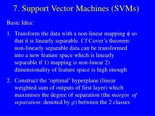
Support Vector Machines (Chapter 7). CS775. History of SVM. SVM is related to statistical learning theory [3] SVM was first introduced in 1992 [1] SVM becomes popular because of its success in handwritten digit recognition

E N D
History of SVM • SVM is related to statistical learning theory [3] • SVM was first introduced in 1992 [1] • SVM becomes popular because of its success in handwritten digit recognition • 1.1% test error rate for SVM. This is the same as the error rates of a carefully constructed neural network, LeNet 4. • See Section 5.11 in [2] or the discussion in [3] for details • SVM is now regarded as an important example of “kernel methods”, one of the key area in machine learning [1] B.E. Boser et al. A Training Algorithm for Optimal Margin Classifiers. Proceedings of the Fifth Annual Workshop on Computational Learning Theory 5 144-152, Pittsburgh, 1992. [2] L. Bottou et al. Comparison of classifier methods: a case study in handwritten digit recognition. Proceedings of the 12th IAPR International Conference on Pattern Recognition, vol. 2, pp. 77-82. [3] V. Vapnik. The Nature of Statistical Learning Theory. 2nd edition, Springer, 1999.
Class 2 Class 1 What is a good Decision Boundary? • Consider a two-class, linearly separable classification problem • Many decision boundaries! • The Perceptron algorithm can be used to find such a boundary • Different algorithms have been proposed • Are all decision boundaries equally good?
a Linear Classifiers x f yest f(x,w,b) = sign(w. x+ b) denotes +1 denotes -1 Any of these would be fine.. ..but which is best?
Examples of Bad Decision Boundaries Class 2 Class 2 Class 1 Class 1
a Classifier Margin x f yest f(x,w,b) = sign(w. x+ b) denotes +1 denotes -1 Define the margin of a linear classifier as the width that the boundary could be increased by before hitting a datapoint.
a Maximum Margin x f yest f(x,w,b) = sign(w. x+ b) denotes +1 denotes -1 The maximum margin linear classifier is the linear classifier with the, um, maximum margin. This is the simplest kind of SVM (Called an LSVM) Linear SVM
a Maximum Margin x f yest f(x,w,b) = sign(w. x- b) denotes +1 denotes -1 The maximum margin linear classifier is the linear classifier with the, um, maximum margin. This is the simplest kind of SVM (Called an LSVM) Support Vectors are those datapoints that the margin pushes up against Linear SVM
Why Maximum Margin? • Intuitively this feels safest. • If we’ve made a small error in the location of the boundary (it’s been jolted in its perpendicular direction) this gives us least chance of causing a misclassification. • LOOCV is easy since the model is immune to removal of any non-support-vector datapoints. • There’s some theory (using VC dimension) that is related to (but not the same as) the proposition that this is a good thing. • Empirically it works very very well. f(x,w,b) = sign(w. x- b) denotes +1 denotes -1 The maximum margin linear classifier is the linear classifier with the, um, maximum margin. This is the simplest kind of SVM (Called an LSVM) Support Vectors are those datapoints that the margin pushes up against
Large-margin Decision Boundary • The decision boundary should be as far away from the data of both classes as possible • We should maximize the margin, m • Distance between the origin and the line wtx=k is k/||w|| Class 2 m Class 1
Finding the Decision Boundary • Let {x1, ..., xn} be our data set and let yiÎ {1,-1} be the class label of xi • The decision boundary should classify all points correctly Þ • The decision boundary can be found by solving the following constrained optimization problem • This is a constrained optimization problem. Solving it requires some new tools
Recap of Constrained Optimization • Suppose we want to: minimize f(x) subject to g(x) = 0 • A necessary condition for x0 to be a solution: • a: the Lagrange multiplier • For multiple constraints gi(x) = 0, i=1, …, m, we need a Lagrange multiplier ai for each of the constraints
Recap of Constrained Optimization • The case for inequality constraint gi(x)£0 is similar, except that the Lagrange multiplier ai should be positive • If x0 is a solution to the constrained optimization problem • There must exist ai³0 for i=1, …, m such that x0 satisfy • The function is also known as the Lagrangrian; we want to set its gradient to 0
Back to the Original Problem • The Lagrangian is • Note that ||w||2 = wTw • Setting the gradient of w.r.t. w and b to zero, we have
Ready for the kernel trick! The Dual Problem • If we substitute to , we have • Note that • This is a function of ai only
The Dual Problem • The new objective function is in terms of ai only • It is known as the dual problem: if we know w, we know all ai; if we know all ai, we know w • The original problem is known as the primal problem • The objective function of the dual problem needs to be maximized! • The dual problem is therefore: Properties of ai when we introduce the Lagrange multipliers The result when we differentiate the original Lagrangian w.r.t. b
The Dual Problem • This is a quadratic programming (QP) problem • A global maximum of ai can always be found • w can be recovered by
Karush-Kuhn-Tucker conditions Karush-Kuhn-Tucker conditions
Points that push against the margin (support vectors) – the only ones with For our problem Any other point (not a support vector)
Consequently… • The only points with positive Lagrange coefficients are support vectors • The other points play no role (they don’t add anything to the evaluation) • You only need to retain support vectors, once the model is trained! (Huge savings!)
The Quadratic Programming Problem • Many approaches have been proposed • Loqo, cplex, etc. (see http://www.numerical.rl.ac.uk/qp/qp.html) • Most are “interior-point” methods • Start with an initial solution that can violate the constraints • Improve this solution by optimizing the objective function and/or reducing the amount of constraint violation • For SVM, sequential minimal optimization (SMO) seems to be the most popular • A QP with two variables is trivial to solve • Each iteration of SMO picks a pair of (ai,aj) and solve the QP with these two variables; repeat until convergence • In practice, we can just regard the QP solver as a “black-box” without bothering how it works
A Geometrical Interpretation Class 2 a10=0 a8=0.6 a7=0 a2=0 a5=0 a1=0.8 a4=0 a6=1.4 a9=0 a3=0 Class 1
Class 2 Class 1 Overlapping: Non-linearly Separable Problems • We allow “error” xi in classification; it is based on the output of the discriminant function wTx+b • xi approximates the number of misclassified samples
Soft Margin Hyperplane • If we minimize åixi, xi can be computed by • xi are “slack variables” in optimization • Note that xi=0 if there is no error for xi • xi is an upper bound of the number of errors • We want to minimize • C : tradeoff parameter between error and margin • The optimization problem becomes
The Optimization Problem • The dual of this new constrained optimization problem is • w is recovered as • This is very similar to the optimization problem in the linear separable case, except that there is an upper bound C on ai now • Once again, a QP solver can be used to find ai
KKT conditions Only support vectors have positive alphas (discard the rest!) KKT If then the point is on the margin! Else The point is inside the margin
Extension to Non-linear Decision Boundary • So far, we have only considered large-margin classifier with a linear decision boundary • How to generalize it to become nonlinear? • Key idea: transform xi to a higher dimensional space to “make life easier” • Input space: the space the point xi are located • Feature space: the space of f(xi) after transformation • Why transform? • Linear operation in the feature space is equivalent to non-linear operation in input space • Classification can become easier with a proper transformation. In the XOR problem, for example, adding a new feature of x1x2 make the problem linearly separable
f( ) f( ) f( ) f( ) f( ) f( ) f( ) f( ) f( ) f( ) f( ) f( ) f( ) f( ) f( ) f( ) f( ) f( ) Transforming the Data • Computation in the feature space can be costly because it is high dimensional • The feature space can be infinite-dimensional! • The kernel trick comes to rescue f(.) Feature space Input space Note: feature space is of higher dimension than the input space in practice
The Kernel Trick • Recall the SVM optimization problem • The data points only appear as inner product • As long as we can calculate the inner product in the feature space, we do not need the mapping explicitly • Many common geometric operations (angles, distances) can be expressed by inner products • Define the kernel function K by
An Example for f(.) and K(.,.) • Suppose f(.) is given as follows • An inner product in the feature space is • So, if we define the kernel function as follows, there is no need to carry out f(.) explicitly • This use of kernel function to avoid carrying out f(.) explicitly is known as the kernel trick
Kernel Functions • In practical use of SVM, the user specifies the kernel function; the transformation f(.) is not explicitly stated • Given a kernel function K(xi, xj), the transformation f(.) is given by its eigenfunctions (a concept in functional analysis) • Eigenfunctions can be difficult to construct explicitly • This is why people only specify the kernel function without worrying about the exact transformation • Another view: kernel function, being an inner product, is really a similarity measure between the objects
Examples of Kernel Functions • Polynomial kernel with degree d • Radial basis function kernel with width s • Closely related to radial basis function neural networks • The feature space is infinite-dimensional • Sigmoid with parameter k and q • It does not satisfy the Mercer condition on all k and q
Original With kernel function Modification Due to Kernel Function • Change all inner products to kernel functions • For training,
Original With kernel function Modification Due to Kernel Function • For evaluation, the new data z is classified as class 1 if f ³0, and as class 2 if f <0
The parameter C for non-linear SVMs • Perfect separation of training data can, in general be achieved in the enlarged feature space F • Such perfect separation is actually bad: it leads to the danger of overfitting the data. Then the classifier will generalize poorly. • A proper setting of C allows to avoid overfitting
C in non-linear SVMs • Let’s look once again at the objective function • C is the penalty for errors of misclassification • Large C: discourages any positive parameters tendency to overfit the data highly complicated boundaries in input space • Small C: encourages a small value of ||w|| larger margin more data on the wrong side of the margin smoother decision boundary in input space • In practice: tune C to achieve best performance
Alternative formulation of soft margin problems • Due to Schölkopf et al Lower bound on the fraction of support vectors Upper bound on the fraction of margin errors
More on Kernel Functions • Since the training of SVM only requires the value of K(xi, xj), there is no restriction of the form of xi and xj • xi can be a sequence or a tree, instead of a feature vector • K(xi, xj) is just a similarity measure comparing xi and xj • For a test object z, the discriminat function essentially is a weighted sum of the similarity between z and a pre-selected set of objects (the support vectors)
More on Kernel Functions • Not all similarity measures can be used as kernel function, however • The kernel function needs to satisfy the Mercer function, i.e., the function is “positive-definite” • This implies that the n by n kernel matrix, in which the (i,j)-th entry is the K(xi, xj), is always positive definite • This also means that the QP is convex and can be solved in polynomial time
Example • Suppose we have 5 1D data points • x1=1, x2=2, x3=4, x4=5, x5=6, with 1, 2, 6 as class 1 and 4, 5 as class 2 y1=1, y2=1, y3=-1, y4=-1, y5=1 • We use the polynomial kernel of degree 2 • K(x,y) = (xy+1)2 • C is set to 100 • We first find ai (i=1, …, 5) by
Example • By using a QP solver, we get • a1=0, a2=2.5, a3=0, a4=7.333, a5=4.833 • Note that the constraints are indeed satisfied • The support vectors are {x2=2, x4=5, x5=6} • The discriminant function is • b is recovered by solving f(2)=1 or by f(5)=-1 or by f(6)=1, as x2 and x5 lie on the line and x4 lies on the line • All three give b=9
Example Value of discriminant function class 1 class 1 class 2 1 2 4 5 6
Why SVM Work? • The feature space is often very high dimensional. Why don’t we have the curse of dimensionality? • A classifier in a high-dimensional space has many parameters and is hard to estimate • Vapnik argues that the fundamental problem is not the number of parameters to be estimated. Rather, the problem is about the flexibility of a classifier • Typically, a classifier with many parameters is very flexible, but there are also exceptions • Let xi=10i where i ranges from 1 to n. The classifier can classify all xi correctly for all possible combination of class labels on xi • This 1-parameter classifier is very flexible
Why SVM works? • Vapnik argues that the flexibility of a classifier should not be characterized by the number of parameters, but by the flexibility (capacity) of a classifier • This is formalized by the “VC-dimension” of a classifier • Consider a linear classifier in two-dimensional space • If we have three training data points, no matter how those points are labeled, we can classify them perfectly
VC-dimension • However, if we have four points, we can find a labeling such that the linear classifier fails to be perfect • We can see that 3 is the critical number • The VC-dimension of a linear classifier in a 2D space is 3 because, if we have 3 points in the training set, perfect classification is always possible irrespective of the labeling, whereas for 4 points, perfect classification can be impossible
VC-dimension • The VC-dimension of the nearest neighbor classifier is infinity, because no matter how many points you have, you get perfect classification on training data • The higher the VC-dimension, the more flexible a classifier is • VC-dimension, however, is a theoretical concept; the VC-dimension of most classifiers, in practice, is difficult to be computed exactly • Qualitatively, if we think a classifier is flexible, it probably has a high VC-dimension
Structural Risk Minimization (SRM) • A fancy term, but it simply means: we should find a classifier that minimizes the sum of training error (empirical risk) and a term that is a function of the flexibility of the classifier (model complexity) • Recall the concept of confidence interval (CI) • For example, we are 99% confident that the population mean lies in the 99% CI estimated from a sample • We can also construct a CI for the generalization error (error on the test set)