Download

1 / 82
820 likes | 838 Views
Fixed and Random Effects. Theory of Analysis of Variance. [ e 2 + k t 2 ]/ e 2 = 1, if k t 2 = 0. Setting Expected Mean Squares. The expected mean square for a source of variation (say X) contains. the error term. a term in 2 x.

E N D
Theory of Analysis of Variance [e2 + kt2]/e2 = 1, if kt2 = 0
Setting Expected Mean Squares • The expected mean square for a source of variation (say X) contains. • the error term. • a term in 2x. • a variance term for other selected interactions involving X.
Coefficients for EMS Coefficient for error mean square is always 1 Coefficient of other expected mean squares is # reps times the product of factors levels that do not appear in the factor name.
Expected Mean Squares • Which interactions to include in an EMS? • All the factors appear in the interaction. • All the other factors in the interaction are Random Effects.
Multiple Comparisons • Multiple Range Tests: • t-tests and LSD’s; • Tukey’s and Duncan’s. • Orthogonal Contrasts.
Multiple t-Test sed[x] = (22/n) (2 x 94,773/4) |XA - XB|/sed[x] >= tp/2
Least Significant Difference |XA - XB|/sed[x] >= tp/2 LSD = tp/2 x sed[x] t0.025 = 2.518 LSD = 2.518 x 217.7 = 548.2
Least Significant Difference Say one of the cultivars (E) is a control check and we want to ask: are any of the others different from the check? LSD = 2.518 x 217.7 = 548.2 XE+ LSD 1796 + 548.2 = 2342.2 to 1247.80
Means and Rankings Range = 1796 + 548.2 = 2342.2 to 1247.80
Tukey’s Multiple Range Test W = q(p,f) x se[x] se[x] = (2/n) (94,773/4) = 153.9 W = 4.64 x 153.9 = 714.1
Consider that cultivars A and B were developed in Idaho and C and D developed in California • Do the two Idaho cultivars have the same yield potential? • Do the two California cultivars have the same yield potential? • Are Idaho cultivars higher yielding than California cultivars?
Orthogonality ci = 0 [c1i xc2i] = 0 -1 -1 +1 +1 -- ci = 0 -1 +1 -1 +1 -- ci = 0 +1 -1 -1 +1 -- ci = 0
Calculating Orthogonal Contrasts d.f. (single contrast) = 1 S.Sq(contrast) = M.Sq = [ci x Yi]2/nci2]
S.Sq = [cix Yi]/[n ci2] S.Sq(1) [(-1)64.1+(-1)76.6+(1)40.1+(1)47.8]2/ n ci2 = 52.82/(3x4) = 232.32
S.Sq(2) [(-1)x64.1+(+1) x 76.6]2/(3x2) 26.04 S.Sq(3) [(-1)x40.1+(+1) x 47.8]2/(3x2) 9.88
Orthogonal Contrasts • Five dry bean cultivars (A, B, C, D, and E). • Cultivars A and B are drought susceptible. • Cultivars C, D and E are drought resistant. • Four Replicate RCB, one location • Limited irrigation applied.
Orthogonal Contrasts • Is there any difference in yield potential between drought resistant and susceptible cultivars? • Is there any difference in yield potential between the two drought susceptible cultivars? • Are there any differences in yield potential between the three drought resistant cultivars?
S.Sq(1)=[(-3)130+(-3)124+(2)141+(2)186+(2)119]2 /nci2 1302/(4x40) = 140.8 S.Sq(2)=[(-1)130+(+1)124]2 /nci2 62/(4x2) = 4.5 S.Sq(Rem) = S.Sq(Cult)-S.Sq(1)-S.Sq(2) 728.2-140.8-4.5 = 582.9 (with 2 d.f.)
S.Sq(1)=[(-3)130+(-3)124+(2)141+(2)186+(2)119]2 /nci2 1302/(4x40) = 140.8 S.Sq(2)=[(-1)130+(-1)124+(-1)141+(4)186+(-1)119]2 /nci2 2302/(4x20) = 661.2 S.Sq(Rem) = S.Sq(Cult)-S.Sq(1)-S.Sq(2) 728.2-140.8-661.2 = -73.8 (Oops !!!) (with 2 d.f.)
Orthogonality c1i = 0 (-3) + (-3) + (+2) + (+2) + (+2) = 0 = c2i = 0 (-1) + (-1) + (-1) + (+4) + (-1) = 0 = [c1i x c2i] = 0 (-3)(-1)+(-3)(-1)+2(-1)+2(4)+2(-1) =10 =