Download
1 / 20
200 likes | 209 Views
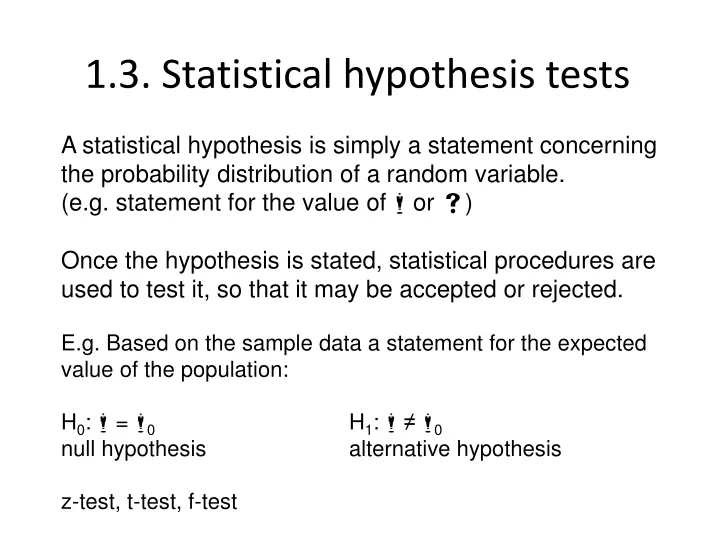
1.3. Statistical hypothesis tests. A statistical hypothesis is simply a statement concerning the probability distribution of a random variable. (e.g. statement for the value of m or s )

E N D
1.3. Statistical hypothesis tests A statistical hypothesis is simply a statement concerning the probability distribution of a random variable. (e.g. statement for the value of m or s) Once the hypothesis is stated, statistical procedures are used to test it, so that it may be accepted or rejected. E.g. Based on the sample data a statement for the expected value of the population: H0: m = m0 H1: m ≠ m0 null hypothesis alternative hypothesis z-test, t-test, f-test
z-test The population variance s2 is known from former experiments. Hence the standard normal distribution (z-distribution) can be used. It is tested that m is equal to a value m0: H0: m = m0 H1: m ≠ m0 null hypothesis alternative hypothesis (two-sided) test statistic: If is too far from then H0 is rejected.
Steps of the z-test Example 1-9. The weight of an object was determined with 4 measurements. The sample average is . The population variance s2 is known from former experiments: 10-4 g2. Can we conclude that the observation is from a population having the expected value of 5.0000 g (the real weight of the object)? - Hypotheses H0: m = m0 =5.0000 g H1: m ≠ m0 • Test statistic: • Critical region for the test statistic at the chosen significance level (e.g. a = 0.05; 1 – a = 0.95) : za/2 = ? It can be obtained from a table.
From table: za/2 = 1.96 critical region accepted critical region • Accept or reject H0 by comparing the calculated value of the test statistic with the critical region. In this example H0 is accepted at significance level 0.05 since 1.84<1.96 (It can be concluded from the measured data that the expected value is 5.0000 g.) https://www.socscistatistics.com/tests/
Example 1-10. The maximum content of impurities in a chemical is 5.0000 g. The mean of 4 measurements . The population variance s2 is known from former experiments: 10-4 g2. Can we conclude that the impurity content doesn’t exceed the limit of 5.0000 g? - Hypotheses H0: m ≤ m0 =5.0000 g H1: m > m0 (one-sided) • Test statistic: - significance level: a = 0.05; 1 – a = 0.95 From table: za = 1.645 1.84 > 1.645 hence the hypothesis is rejected
z0 = 1.84; za = 1.645 The null hypothesis is rejected, because the value of the z0 test statistic is so large, that it would happen at random with a probability less than a.
t-test It can test (similarly to the z-test) whether the mean of a population has a value specified in a null hypothesis. The population variance s2 is not known from former experiments. Hence the t-distribution can be used. H0: m = m0 H1: m ≠ m0 null hypothesis alternative hypothesis (two-sided) test statistic: If t0 is in the critical region then H0 is rejected.
Example 1-11. Suppose that we have made 11 runs on a pilot-plant reactor at constant conditions and have obtained the following values of the percentage yield of desired product: 32, 55, 58, 59, 59, 60, 63, 63, 63, 63, 67. Test the hypothesis that m=63. (avr = 58.36; s = 9.33) Example 1-12. The desired minimal concentration of a reagent is 99%. Is the specification met if the measured values are: 98.3 97.3 97.5 (Let the level of significance a = 0.05) Example 1-13. 500 gr mass must be filled into the tins in a factory. Because of the unevenness of the filler machine sometimes a little more, sometimes a little less is filled than 500 gr. Can we conclude that the machine works properly if the measured weights are: 483, 502, 498, 496, 502, 483, 494, 491, 505, 486.
Unpaired (independent) two-sample t-test Two independent sets of samples are obtained from two populations to compare the means of the populations. The variances of the two populations are assumed to be equal. It must be checked by F-test! s: pooled standard deviation The t statistic to test whether the means are different: Degree of freedom: n = n1 + n2 – 2
Null hypothesis: Test statistic: If: then we may accept the hypothesis H0 that the means for each population are not different significantlyat level a.
Example 1-14. The weights of the products made by a machine were measured on two different days. The following values were obtained: Using the level of significance a = 0.05 determine whether the mean weight of the products of day1 is different from that of day2? Are the variances of the two population equal? F-test: From F-table: F0.05(9, 14) = 2.65; 1.333 < 2.65, hence the variances can be accepted to be equal.
Since 3.7 > 2.069, we reject H0 at a=0.05. The difference between the two days is significant at the 0.05 level.
Paired t-test Consists of a sample of matched pairs (xi, yi). E.g. blood pressure values before and after treatment. Test statistic:
Example 1-15. An experiment is conducted on the effect of alcohol on perceptual motor ability. Ten subjects are each tested twice, once after having two drinks and once after having two glasses of water. The two tests were on two different days to give the alcohol a chance to wear off. The scores of the 10 subjects are shown below. Higher scores reflect better performance. Test to see if alcohol had a significant effect. Use 0.01 significance level!
Test statistic: Since 5.01 > 3.250, we reject H0 at a=0.01. The alcohol had significant effect at the 0.01 level.
Example 1-16. The wear of two kinds of raw material (A and B) is compared as shoe soles on the foot of 10-10 boys. Is the difference of means significant at α=0.05 level?
Example 1-17. The wear of two kinds of raw material (A and B) is compared as shoe soles on the left and right (randomly) foot of 10 boys. Is the difference of means significant at α=0.05 level?
Example 1-18. The overall distance traveled by a golf ball is tested by hitting the ball with a mechanical golfer. Ten-ten randomly selected balls of two different brands are tested and the overall distance measured. The data follow: Brand 1: 275, 286, 287, 271, 283, 271, 279, 275, 263, 267 (s2=64.46, avg=275.7) Brand 2: 258, 244, 260, 265, 273, 281, 271, 270, 263, 268 (s2=100.90, avg=265.3) Test the hypothesis that both brands of ball have equal mean overall distance. Use alpha equals to 0.05.
Example 1-19. Two different analytical tests can be used to determine the impurity level in steel alloys. Eight specimens are tested using both procedures, and the results are shown in the following tabulation. Are the two analytical methods biased to each other? Use 0.05 significance level.