Download
1 / 32
410 likes | 919 Views
In the Name of the Most High . Stochastic Processes. Behzad Akbari Spring 2009 Tarbiat Modares University. These slides are based on the slides of Prof. K.S. Trivedi (Duke University). What is a stochastic process?. Stochastic Process Characterization.

E N D
In the Name of the Most High Stochastic Processes Behzad Akbari Spring 2009 Tarbiat Modares University These slides are based on the slides of Prof. K.S. Trivedi (Duke University)
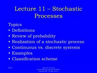
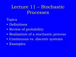
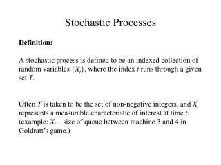
Stochastic Process Characterization • At a fixed time t=t1, we can define X(t1). Similarly, we can define, X(t2), .., X(tk). • X(t1) can be characterized by its distribution function, • We can also consider the joint distribution function, • Discrete and continuous cases: • Index set T may be discrete/continuous • State space I (i.e. sample space S) may be discrete/continuous
Classification of Stochastic Processes • Four classes of stochastic processes: • Discrete-state process chain • discrete-time process stochastic sequence {Xn | n є T} (e.g., probing a system every 10 ms.)
Example: a Queuing System • Inter arrival times Y1, Y2, … (mutually independent) (FY) • Service times: S1, S2, … (mutually independent) (FS) • Notation for a queuing system: Fy /FY /m • Possible arrival/service time distributions types are: • M: Memory-less (i.e., EXP) • D: Deterministic • G: General distribution • Ek: k-stage Erlang etc. • M/M/1 Memory-less arrival/departure processes with 1-service station • Some examples: M/M/1, M/G/1, M/M/k, M/D/1
Discrete time, Discrete space Stochastic Processes • Nk: Number of jobs waiting in the system at the time of kth job’s departure Stochastic process {Nk|k=1,2,…}: Nk Discrete k Discrete
Continuous Time, Discrete Space • X(t): Number of jobs in the system at time t. {X(t)|t є T} forms a continuous-time, discrete-state stochastic process, with, X(t) Discrete Continuous
Discrete Time, Continuous Space • Wk: wait time for the kth job. Then {Wk| k є T}forms a Discrete-time, Continuous-state stochastic process, where, Wk Continuous k Discrete
Continuous Time, Continuous Space • Y(t): total service time for all jobs in the system at time t. Y(t) forms a continuous-time, continuous-state stochastic process, Where, Y(t) t
Further Classification • Similarly, we can define nth order distribution: • Difficult to compute nth order distribution. • Can the nth order distribution computations be simplified? • Yes. Under some simplifying assumptions: • Stationary (strict) • F(x;t) = F(x;t+τ) all moments are time-invariant (1st order distribution) (2nd order distribution)
Independent and Renewal Process • Independence • As consequence of independence, we can define Renewal Process • Discrete time independent process {Xn|n=1,2,…} (X1, X2, .. are iid, non-negative rvs), e.g., repair/replacement after a failure.
Markov Chain Sojourn time • Let, Y: time spent in a given state • Y is also called the sojourn time and has memoryless property: • This result says that for a homogeneous discrete time Markov chain, sojourn time in a state follows EXP( ) distribution. • Semi-Markov process is one in which the sojourn time in state may not be EXP( ) distributed.
Bernoulli & Binomial Processes • A set of Bernoulli sequences, {Yi|i=1,2,3,..}, Yi =1 or 0 • {Yi} forms a Bernoulli Process. Often Yi’s are independent. • E[Yi] = p; E[Yi2] = p; Var[Yi] = p(1-p) • Define another stochastic process , {Sn|n=1,2,3,..}, where Sn = Y1 +Y2 +…+ Yn (i.e. Sn :sequence of partial sums) • Sn = Sn-1+ Yn (recursive form) • P[Sn = k| Sn-1= k] = P[Yn = 0] = (1-p)and, • P[Sn = k| Sn-1= k-1] = P[Yn = 1] = p • {Sn |n=1,2,3,..}, forms a Binomial process • P[Sn = k] =
Poisson Process • A continuous time, discrete state process. • N(t): no. of events occurring in time (0, t]. Events may be, • # of packets arriving at a router port • # of incoming telephone calls at a switch • # of jobs arriving at file/computer server • Number of failed components in time interval • Events occurs successively and that intervals between these successive events are iid rvs, each following EXP( ) • λ: average arrival rate (1/ λ: average time between arrivals) • λ: average failure rate (1/ λ: average time between failures)
Poisson Process (contd.) • N(t) forms a Poisson process provided: • N(0) = 0 • Events within non-overlapping intervals are independent • In a very small interval h, only one event may occur (prob. p(h)) • Letting, pn(t) = P[N(t)=n], • Hence, for a Poisson process, interval arrival times follow EXP( ) (memory-less) distribution. Such a Poisson process is non-stationary. • Mean = Var = λt ; What about E[N(t)/t], as t infinity?
Merged Multiple Poisson Process Streams • Consider the system, • Proof: Using z-transform. Letting, α = λt, +
Decomposing a Poisson Process Stream • Decompose a Poisson process into multiple streams • N arrivals decomposed into {n1, n2, .., nk}; N= n1+n2, ..,+nk • Cond. pmf • Since, • The uncond. pmf +
Renewal Counting Process • Poisson process EXP( ) distributed inter-arrival times. • What if the EXP( ) assumption is removed renewal proc. • Renewal proc. : {Xi|i=1,2,…} (Xi’s are iid non-EXP rvs) • Xi : time gap between the occurrence of ith and (i+1)st event • Sk = X1 + X2 + .. + Xk time to occurrence of the kth event. • N(t)- Renewal counting process is a discrete-state, continuous-time stochastic. N(t) denotes no. of renewals in the interval (0, t].
Renewal Counting Processes (contd.) Sn t • For N(t), what is P(N(t) = n)? • nth renewal takes place at time t (account for the equality) • If the nth renewal occurs at time tn < t, then one or more renewals occur in the interval (tn < t]. tn More arrivals possible
Renewal Counting Process Expectation • Let, m(t) = E[N(t)]. Then, m(t) = mean no. of arrivals in time (0,t]. m(t) is called the renewal function.
Renewal Density Function • Renewal density function: • For example, if the renewal interval X is EXP(λ x), then • d(t) = λ , t >= 0 and m(t) = λ t , t >= 0. • P[N(t)=n] = • Fn(t) will turn out to be e–λ t (λ t)n/n! i.e Poissonprocess pmf n-stage Erlang
Availability Analysis • Availability: is defined is the ability of a system to provide the desired service. • If no repairs/replacements, Availability = Reliability. • If repairs are possible, then above def. is pessimistic. • MTBF = E[Di+Ti+1] = E[Ti+Di]=E[Xi]=MTTF+MTTR MTBF T1 D1 T2 D2 T3 D3 T4 D4 …….
Availability Analysis (contd.) • Two mutually exclusive situations: • System does not fail before time t A(t) = R(t) • System fails, but the repair is completed before time t • Therefore, A(t) = sum of these two probabilities renewal Repair is completed with in this interval t x
Availability Expression • dA(x) : Incremental availability • dA(x) = Prob(that after renewal, life time is > (t-x) & that the renewal occurs in the interval (x,x+dx]) Repair is completed within this interval x t x+dx 0 Renewed life time >= (t-x)
Availability Expression (contd.) • A(t) can also be expressed in the Laplace domain. • Since, R(t) = 1-W(t) or LR(s) = 1/s – LW(s) = 1/s –Lw(s)/s • What happens when t becomes very large? • However,
Availability, MTTF and MTTR • Steady state availability A is: • for small values of s,
Availability Example • Assuming EXP( ) density fn for g(t) and w(t)