Download
1 / 36
360 likes | 524 Views
Descriptive Statistics and the Normal Distribution. HPHE 3150 Dr. Ayers. Introduction Review. Terminology Reliability Validity Objectivity Formative vs Summative evaluation Norm- vs Criterion-referenced standards. Scales of Measurement. Nominal name or classify

E N D
Descriptive Statistics and theNormal Distribution HPHE 3150 Dr. Ayers
Introduction Review • Terminology • Reliability • Validity • Objectivity • Formative vs Summative evaluation • Norm- vs Criterion-referenced standards
Scales of Measurement • Nominal • name or classify • Major, gender, yr in college • Ordinal • order or rank • Sports rankings • Continuous • Interval equal units, arbitrary zero • Temperature, SAT/ACT score • Ratio equal units, absolute zero (total absence of characteristic) • Height, weight
Summation Notation • Sis read as "the sum of" • X is an observed score • N = the number of observations • Complete ( ) operations first • Exponents then * and / then + and -
Operations Orders 65 26 -5 4 2 -3
Summation Notation Practice:Mastery Item 3.2 Scores: 3, 1, 2, 2, 4, 5, 1, 4, 3, 5 Determine: ∑ X (∑ X)2 ∑ X2 30 900 110
Percentile • The percent of observations that fall at or below a given point • Range from 0% to 100% • Allows normative performance comparisons • If I am @ the 90th percentile, • how many folks did better than me?
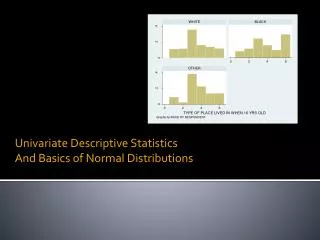
Test Score Frequency Distribution Figure 3.1 (p.42 explanation)
Central Tendency Where do the scores tend to center? • Meansum scores / # scores • Median (P50)exact middle of ordered scores • Mode most frequent score
Raw scores 2 7 5 5 1 Rank order 1 2 5 5 7 • Mean • Median (P50) • Mode • Mean: 4 (20/5) • Median: 5 • Mode: 5
Distribution Shapes Figure 3.2So what? OUTLIERS Direction of tail = +/-
Three Symmetrical Curves Figure 3.3 The difference here is the variability; Fully normal More heterogeneous More homogeneous
Descriptive Statistics I • What is the most important thing you learned today? • What do you feel most confident explaining to a classmate?
Descriptive Statistics IREVIEW • Measurement scales • Nominal, Ordinal, Continuous (interval, ratio) • Summation Notation: 3, 4, 5, 5, 8 Determine: ∑ X, (∑ X)2, ∑X2 9+16+25+25+64 25 625 139 • Percentiles: so what?
Measures of central tendency • 3, 4, 5, 5, 8 • Mean (?), median (?), mode (?) • Distribution shapes
Total variance Variability • RangeHi – Low scores only (least reliable measure; 2 scores only) • Variance (s2) inferential statsSpread of scores based on the squared deviation of each score from mean Most stable measure of variability • Standard Deviation (S) descriptive statsSquare root of the variance Most commonly used measure of variability Error TrueVar-iance
Variance (Table 3.2) The didactic formula 4+1+0+1+4=1010 = 2.5 5-1=4 4 The calculating formula 55 - 225 = 55-45=10 = 2.5 5 4 4 4
Standard Deviation The square root of the variance Nearly 100% scores in a normal distribution are captured by the mean + 3 standard deviations M + S 100 + 10
The Normal Distribution M + 1s = 68.26% of observations M + 2s = 95.44% of observations M + 3s = 99.74% of observations
Calculating Standard Deviation Raw scores 3 7 4 5 1 ∑ 20 Mean: 4 (X-M) -1 3 0 1 -3 0 (X-M)2 1 9 0 1 9 20 S= √20 5 S= √4 S=2
Coefficient of Variation (V)Relative variability Relative variability around the mean ORdetermine homogeneity of two data sets with different units S / M Relative variability accounted for by the mean when units of measure are different (ht, hr, running speed, etc.) Helps more fully describe different data sets that have a common std deviation (S) but unique means (M) Lower V=mean accounts for most variability in scores .1 - .2=homogeneous >.5=heterogeneous
Descriptive Statistics II • What is the “muddiest” thing you learned today?
Descriptive Statistics IIREVIEW Variability • Range • Variance: Spread of scores based on the squared deviation of each score from mean Most stable measure • Standard deviation Most commonly used measure Coefficient of variation • Relative variability around the mean (homogeneity of scores) • Helps more fully describe relative variability of different data sets 50+10 What does this tell you?
Standard ScoresZ or t • Set of observations standardized around a given M and standard deviation • Score transformed based on its magnitude relative to other scores in the group • Converting scores to Z scores expresses a score’s distance from its own mean in sd units • Use of standard scores: determine composite scores from different measures (bball: shoot, dribble); weight?
Standard Scores • Z-score M=0, s=1 • T-scoreT = 50 + 10 * (Z) M=50, s=10 • Percentilep = 50 + Z (%ile)
Conversion to Standard Scores Raw scores 3 7 4 5 1 • Mean: 4 • St. Dev: 2 X-M -1 3 0 1 -3 Z -.5 1.5 0 .5 -1.5 SO WHAT? You have a Z score but what do you do with it? What does it tell you? Allows the comparison of scores using different scales to compare “apples to apples”
Descriptive Statistics II REVIEW Standard Scores • Converting scores to Z scores expresses a score’s distance from its own mean in sd units • Value? Coefficient of variation • Relative variability around the mean (homogeneity of scores) • Helps more fully describe relative variability of different data sets 100+20 What does this tell you? Between what values do 95% of the scores in this data set fall?
Normal-curve Areas Table 3.4 • Z scores are on the left and across the top • Z=1.64: 1.6 on left , .04 on top=44.95 • Since 1.64 is +, add 44.95 to 50 (mean) for 95th percentile • Values in the body of the table are percentage between the mean and a given standard deviation distance • ½ scores below mean, so + 50 if Z is +/- • The "reference point" is the mean • +Z=better than the mean • -Z=worse than the mean
Area of normal curve between 1 and 1.5 std dev above the mean Figure 3.7
Normal curve practice • Z score Z = (X-M)/S • T score T = 50 + 10 * (Z) • Percentile P = 50 + Z percentile(+: add to 50, -: subtract from 50) • Raw scores • Hints • Draw a picture • What is the z score? • Can the z table help?
Descriptive Statistics III • Explain one thing that you learned today to a classmate • What is the “muddiest” thing you learned today?