Download

1 / 50
570 likes | 1.52k Views
External Flows. CEE 331 March 11, 2014. Overview. The F ss connection to Drag Boundary Layer Concepts Drag Shear Drag Pressure Drag Pressure Gradients: Separation and Wakes Drag coefficients Vortex Shedding. F ss : Shear and Pressure Forces. Major losses in pipes. Shear forces:

E N D
External Flows CEE 331 March 11, 2014
Overview • The Fss connection to Drag • Boundary Layer Concepts • Drag • Shear Drag • Pressure Drag • Pressure Gradients: Separation and Wakes • Drag coefficients • Vortex Shedding
Fss: Shear and Pressure Forces Major losses in pipes • Shear forces: • viscous drag, frictional drag, or skin friction • caused by shear between the fluid and the solid surface • function of ___________and ______of object • Pressure forces • pressure drag or form drag • caused by _____________from the body • function of area normal to the flow length surface area Flow expansion losses flow separation Projected area
Non-Uniform Flow • In pipes and channels the velocity distribution was uniform (beyond a few pipe diameters or hydraulic radii from the entrance or any flow disturbance) • In external flows the boundary layer (the flow influenced by the solid object) is always growing and the flow is non-uniform • We need to calculate shear in this non-uniform flow!
Boundary Layer Concepts • Two flow regimes • Laminar boundary layer • Turbulent boundary layer • with laminar sub-layer • Calculations of • boundary layer thickness • Shear (as a function of location on the surface) • Viscous Drag (by integrating the shear over the entire surface)
U U U U is maximum Flat Plate: Parallel to Flow boundary layer thickness to y d x shear Why is shear maximum at the leading edge of the plate?
Laminar Boundary Layer:Shear and Drag Force squareroot Boundary Layer thickness increases with the _______ ______ of the distance from the leading edge of the plate Based on momentum and mass conservation and assumed velocity distribution Integrate along length of plate On one side of the plate!
Laminar Boundary Layer:Coefficient of Drag Dimensional analysis
Transition to Turbulence • The boundary layer becomes turbulent when the Reynolds number is approximately 500,000 (based on length of the plate) • The length scale that really controls the transition to turbulence is the _________________________ boundary layer thickness = Red = 3500
U U Transition to Turbulence U U d y turbulent x Viscous sublayer to This slope (du/dy) controls t0. Transition (analogy to pipe flow)
Grows ____________ than laminar Derived from momentum conservation and assumed velocity distribution Turbulent Boundary Layer: (Smooth Plates) more rapidly x 5/4 Integrate shear over plate 5 x 10⁵ < Rel < 107
Boundary Layer Thickness • Water flows over a flat plate at 1 m/s. How long is the laminar region? x = 0.5 m Grand Coulee
1 x 10⁻³ 5 x 10⁻⁴ 2 x 10⁻⁴ 1 x 10⁻⁴ 5 x 10⁻⁵ 2 x 10⁻⁵ 1 x 10⁻⁵ 5 x 10⁻⁶ 2 x 10⁻⁶ 1 x 10⁻⁶ Turbulent boundary Flat Plate Drag Coefficients rough laminar transitional
Example: Solar Car • Solar cars need to be as efficient as possible. They also need a large surface area for the (smooth) solar array. Estimate the power required to counteract the viscous drag on the solar panel at 40 mph • Dimensions: L: 5.9 m W: 2 m H: 1 m • Max. speed: 40 mph on solar power alone • Solar Array: 1200 W peak rair = 1.22 kg/m3 nair = 14.6 x10⁻⁶ m2/s
scales with ____ (based on _______ similarity) Viscous Drag on Ships • The viscous drag on ships can be calculated by assuming a flat plate with the wetted area and length of the ship Lr3 Froude
Separation and Wakes • Separation often occurs at sharp corners • fluid can’t accelerate to go around a sharp corner • Velocities in the Wake are ______ (relative to the free stream velocity) • Pressure in the Wake is relatively ________ (determined by the pressure in the adjacent flow) small constant
Pressure Gradients: Separation and Wakes Diverging streamlines Van Dyke, M. 1982. An Album of Fluid Motion. Stanford: Parabolic Press.
Adverse Pressure Gradients Streamlines diverge behind object • Increasing pressure in direction of flow • Fluid is being decelerated • Fluid in boundary layer has less ______ than the main flow and may be completely stopped. • If boundary layer stops flowing then separation occurs inertia
Point of Separation • Predicting the point of separation on smooth bodies is beyond the scope of this course. • Expect separation to occur where streamlines are diverging (flow is slowing down) • Separation can be expected to occur around any sharp corners (where streamlines diverge rapidly)
U Flat Plate:Streamlines 3 2 4 0 Point v Cp p 1 ______ ________ ____ 2 ______ ________ ____ 3 ______ ________ ____ 4 ______ ________ ____ 1 Cp = 1 >p0 0 <U >p0 0 < Cp < 1 <p0 >U Cp < 0 <U <p0 Cp < 0 Points outside boundary layer! p in wake is uniform
Application of Bernoulli Equation In air pressure change due to elevation is small U = velocity of body relative to fluid
Flat Plate:Pressure Distribution 3 >U <U Front of plate 2 1 0 Back of plate Cd = 2 1 0.8 0 Cp -1 -1.2
Drag Coefficient of Blunt and Streamlined Bodies • Drag dominated by viscous drag, the body is __________. • Drag dominated by pressure drag, the body is _______. • Whether the flow is viscous-drag dominated or pressure-drag dominated depends entirely on the shape of the body. • This drag coefficient is calculated from a measured value of ____ streamlined bluff Flat plate Fss Bicycle page at Princeton
Drag Coefficient at High Reynolds Numbers • Figures 9.28-9.30 bodies with drag coefficients on p 593-595 in text. • hemispherical shell 0.38 • hemispherical shell 1.42 • cube 1.1 • parachute 1.4 Why? Velocity at separation point determines pressure in wake. ? Vs The same!!!
SUVs have got Drag… • Ford Explorer 2002 Cd = 0.41
Automobile Drag Coefficients (High Reynolds Number) Cd = 0.32 Height = 1.539 m Width = 1.775 m Length = 4.351 m Ground clearance = 15 cm 100 kW at 6000 rpm Max speed is 124 mph Where does separation occur? Calculate the power required to overcome drag at 60 mph and 120 mph. What is the projected area?
Electric Vehicles • Electric vehicles are designed to minimize drag. • Typical cars have a coefficient drag of 0.30-0.40. • The EV1 has a drag coefficient of 0.19. Smooth connection to windshield Plan view of car?
Velocity and Drag: Spheres General relationship for submerged objects Spheres only have one shape and orientation! Where Cd is a function of Re
Sphere Terminal Fall Velocity (continued) General equation for falling objects Relationship valid for spheres
Drag Coefficient on a Sphere 1000 Stokes Law 100 Drag Coefficient 10 1 0.1 0.1 1 10 102 103 104 105 106 107 Re=500000 Reynolds Number Turbulent Boundary Layer
Drag Coefficient for a Sphere:Terminal Velocity Equations Valid for laminar and turbulent Laminar flow R < 1 Transitional flow 1 < R < 104 Fully turbulent flow R > 104
Example Calculation of Terminal Velocity Determine the terminal settling velocity of a cryptosporidium oocyst having a diameter of 4 mm and a density of 1.04 g/cm3 in water at 15°C. Reynolds
Drag on a Golf Ball • Drag on a golf ball comes mainly from pressure drag. The only practical way of reducing pressure drag is to design the ball so that the point of separation moves back further on the ball. • The golf ball's dimples increase the turbulence in the boundary layer, increase the _______ of the boundary layer, and delay the onset of separation. • What is the Reynolds number where the boundary layer begins to become turbulent with a golf ball? _________ • Why not use this for aircraft or cars? inertia 40,000 Boundary layer is already turbulent
At what velocity is the boundary layer laminar for an automobile?
Effect of Turbulence Levels on Drag • Flow over a sphere with a trip wire. Causes boundary layer to become turbulent Re=30,000 Re=15,000 Point of separation
Effect of Boundary Layer Transition Real (viscous) fluid: laminar boundary layer Real (viscous) fluid: turbulent boundary layer Ideal (non viscous) fluid Increased inertia in boundary layer No shear!
Spinning Spheres • What happens to the separation points if we start spinning the sphere? LIFT!
Vortex Shedding • Vortices are shed alternately from each side of a cylinder • The separation point and thus the resultant drag force oscillates • Frequency of shedding (n) given by Strouhal number S • S is approximately 0.2 over a wide range of Reynolds numbers (100 - 1,000,000)
Summary: External Flows • Spatially varying flows • boundary layer growth • Example: Spillways • Two sources of drag (Fss) • shear (surface area of object) • pressure (projected area of object) • Separation and Wakes • Interaction of viscous drag and adverse pressure gradient
Challenge • I’m going on vacation and I can’t back all of our luggage in my Matrix. Should I put it on the roof rack or on the hitch?
Challenges • How long would L have to be to double the drag of a sphere? L V=30 m/s D = 3 m
Challenges • How long would L have to be to double the drag of a sphere? D = 3 m V=30 m/s L Find drag of sphere Guess at Re for plate Find drag coefficient for plate(note different area) Solve for L
Elongated sphere D = 3 m V=30 m/s L
Solution: Solar Car U = 17.88 m/s l = 5.9 m nair = 14.6 x 10⁻⁶ m2/s rair = 1.22 kg/m3 Rel = 7.2 x 10⁶ Cd = 3 x 10⁻³ Fd =14 N A = 5.9 m x 2 m = 11.8 m2 P =F*U=250 W
Reynolds Number Check R = 1.1 x 10⁻⁶ R<<1 and therefore in Stokes Law range
Solution: Power a Toyota Matrix at 60 or 120 mph P = 9.3 kW at 60 mph P = 74 kW at 120 mph
Grand Coulee Dam Turbulent boundary layer reaches surface!
Reflections on Drag • What are 3 similarities with Moody diagram? • Laminar • Smooth • Rough • Why 2 curves for smooth (red and green) • Fully turbulent boundary layer • Transition between laminar and turbulent on the plate • Why more detail in transition region here than in Moody diagram? • Are any lines missing on the graph? Function of conditions at leading edge
Drexel SunDragon IV http://cbis.ece.drexel.edu/SunDragon/Cars.html • Vehicle ID: SunDragon IV (# 76)Dimensions: L: 19.2 ft. (5.9 m) W: 6.6 ft. (2 m) H: 3.3 ft. (1 m) Weight: 550 lbs. (249 kg)Solar Array: 1200 W peak; 8 square meters terrestrial grade solar cells; manf: ASE AmericasBatteries: 6.2 kW capacity lead-acid batteries; manf: US BatteryMotor: 10 hp (7.5 kW) brushless DC; manf: Unique MobilityRange: Approximately 200 miles (at 35 mph on batteries alone)Max. speed: 40 mph on solar power alone, 80 mph on solar and battery power.Chassis: Graphite monocoque (Carbon fiber, Kevlar, structural glass, Nomex)Wheels: Three 26 in (66 cm) mountain bike, custom hubsBrakes: Hydraulic disc brakes, regenerative braking (motor)