Download
1 / 53
540 likes | 827 Views
ASKAP. John Bunton ASKAP Project Engineer Japan SKA Workshop 4-5 Nov 20010. Long and storied history of radio-astronomy Scientific and technical capability in research & industry. Australian Radio Astronomy . Parkes 64m - 1961. Sea Cliff Interferometer - 1948. ASKAP Program Goals.

E N D
ASKAP John Bunton ASKAP Project Engineer Japan SKA Workshop 4-5 Nov 20010
Long and storied history of radio-astronomy Scientific and technical capability in research & industry Australian Radio Astronomy Parkes 64m - 1961 Sea Cliff Interferometer - 1948
ASKAP Program Goals Australian SKA Pathfinder Telescope Develop SKA technologies demonstrating wide field-of-view high-dynamic range performance on a world-class array. Murchison Radio Observatory Protect and develop the Murchison Radio Observatory (MRO). SKA Participate fully in prepSKA and advance the full SKA. Support Provide support for other experiments at the MRO (currently MWA, PAPER, CORE, EDGES)
ASKAP Design Specification A sensitive wide field-of-view telescope Number of dishes 36 Dish diameter 12 m Max baseline 6km Resolution 10” (6km array), 30” (2km core) Sensitivity 70 m2/K Field of View 30 deg2 Speed 1.5x10⁵ m4/K2.deg2 Observing frequency 700 – 1800 MHz Processed Bandwidth 300 MHz Channels 16k Focal Plane Phased Array 188 elements (94 dual pol) Dish area = 4072m2 630 Pairs of dishes
ASKAP Design Specification A sensitive wide field-of-view telescope Number of dishes 36 Dish diameter 12 m Max baseline 6km Resolution 10” (6km array), 30” (2km core) Sensitivity 70 m2/K Field of View 30 deg2 Speed 1.5x10⁵ m4/K2.deg2 Observing frequency 700 – 1800 MHz Processed Bandwidth 300 MHz Channels 16k Focal Plane Phased Array 188 elements (94 dual pol) Dish area = 4072m2 630 Pairs of dishes
ASKAP Design Specification A sensitive wide field-of-view telescope Number of dishes 36 Dish diameter 12 m Max baseline 6km Resolution 10” (6km array), 30” (2km core) Sensitivity 70 m2/K Field of View 30 deg2 Speed 1.5x10⁵ m4/K2.deg2 Observing frequency 700 – 1800 MHz Processed Bandwidth 300 MHz Channels 16k Focal Plane Phased Array 188 elements (94 dual pol) Dish area = 4072m2 630 Pairs of dishes
Antenna locations UV coverage (Position of pairs) Fourier Transform for image Resolution eye 60 arc sec Resolution core 30 arc sec Resolution full 10 arc sec Gupta et al. 2008, ATNF ASKAP Memo 21
ASKAP Design Specification A sensitive wide field-of-view telescope Number of dishes 36 Dish diameter 12 m Max baseline 6km Resolution 10” (6km array), 30” (2km core) Sensitivity 70 m2/K Field of View 30 deg2 Speed 1.5x10⁵ m4/K2.deg2 Observing frequency 700 – 1800 MHz Processed Bandwidth 300 MHz Channels 16k Focal Plane Phased Array 188 elements (94 dual pol) Dish area = 4072m2 630 Pairs of dishes
Phased Array Feed Total bandwidth processed = 2.1THz ~200 elements x 36 antennas x 0.3GHz
ASKAP Design Specification A sensitive wide field-of-view telescope Number of dishes 36 Dish diameter 12 m Max baseline 6km Resolution 10” (6km array), 30” (2km core) Sensitivity 70 m2/K Field of View 30 deg2 Speed 1.5x10⁵ m4/K2.deg2 Observing frequency 700 – 1800 MHz Processed Bandwidth 300 MHz Channels 16k Focal Plane Phased Array 188 elements (94 dual pol) Dish area = 4072m2 630 Pairs of dishes
ASKAP Continuum Science • Visible sky to 10 μJy rms • Dec -90 to +30 • Like NVSS/SUMMS but • 40 times deeper • 6 times better resolution shallow Uncharted Phase-space deep \
ASKAP Survey Science Proprams • WALLABY (Koribalski/Staveley-Smith) All sky HI survey to z~0.2 • EMU (Norris) All sky continuum to 10 uJy rms • GASKAP (Dickey) Galactic and Magellanic HI and OH • VAST (Murphy/Chatterjee) Transients and variables (>5 sec) • CRAFT (Dodson/Macquart) Fast transients (<5 sec) • FLASH (Sadler) HI absorption to z~1 • POSSUM (Gaensler/Landecker/Taylor) Polarization / RM grid • DINGO (Meyer) Deep HI emission survey • COAST (Stairs) Pulsar timing and searching • VLBI (Tingay) ASKAP as part of the LBA
ASKAP Location Boolardy Geraldton
Regulation of RFI Geraldton
Low Population Density gazetted towns: 0 population: “up to 160” Geraldton
Australian Strengths gazetted towns: 0 population: “up to 160” Geraldton
Beamforming Task • At the focus of dish illumination of phase array depends on look angle • See examples • Detect power from phased array and sum • Approx. conjugate match • Do this for up to 36 look angles (beams) • Weights different from beam to beam and are frequency dependent • Focal spot size proportional to λ
What is possible • Scan a single beam across the sky and find the maximum sensitivity at each beam position. • Plot this sensitivity Maximum PAF sensitivity • Result provided by Stuart Hay • For current ASKAP PAF
ASKAP Phased Array Feed Digital beamformer Patches Transmission lines Currents Low-noise amplification and conversion Ground plane Weighted sum of inputs • Connected checkerboard array • Self-complementary screen (Babinet’s principle) • High-impedance, differential • Low noise amplifier NF target 0.3dB
Electromagnetics/Microwave Engineering Patches • Connected checkerboard array • Self-complementary screen (Babinet’s principle) • High-impedance, differential • Low noise amplifier NF target 0.3dB
Digital beamformer LNA Requirements Patches • Connected checkerboard array • Self-complementary screen (Babinet’s principle) • High-impedance, differential • Low noise amplifier NF target 0.3dB Currents Ground plane
ASKAP analogue receiver system Focus Cable wraps Pedestal LNA RF on copper A/D RF gain RF filters Frequency Conversion* *Dual conversion • Frequency conversion and sampler in the pedestal • Analog RF signal transmission over coaxial cable • Dual conversion (superheterodyne) receiver
Packaging • Integrating all the pieces together to yield a cost-effective reliable solution whose form factor fits the system. 6768 of these
BEAMFORMER CORRELATORS
Cross Connect Beamformer • Frequency domain beamformer requires filterbank/FFT ahead of beamforming • After filterbank use cross connect to distribute part of bandwidth to each beamformer module CROSS CONNECT Antenna Central Site
DragonFly Digitiser/Filterbank • Digitiser and filterbank system installed in Pedestal • 188 ports x 0.3GHz = 56GHz • 18 Tops/antenna Virtex-6 LX130T (Coarser filterbanks) 2 Dual channel ADC @ 768MS/s 4 SFP+ Optical 40Gb/s total
Redback Beamforming Redback-2 RTM 12x10Gb/s • Located at central site • Industry standard AdvancedTCA shelf • 19MHz – 188 port beamformer per board • 4 LX240T processing FPGAs per board. • Per antenna • Input data 1.9Tb/s • 27 Tops AdvancedTCA shelf with full cross connect backplane
An SKA solution • ADC combined with coarse filterbank with PAF at focus • This can be done on a single chip – eg Fujitsu high-speed ADC/ASIC • high NRE • Also integrate optical fibre drive • Low power and weight • Space and power limit • Major RFI shielding Optical
RF over Fibre solution • RF over Fibre moves ADC to pedestal or nearby building use RF over Fibre • Up to 10s km • Dynamic range? • Simplifies RFI and weight problems • Integrated ADC/Filterbank/Laser driver still advantageous • ~0.5M ADC channels • Cross connect to beamformers may still be optical to provide isolation
ASKAP data flow FGPA+firmware FGPA+firmware Central site Boolardy Correlations to image (grid and 2D FFT) Supercomputer Perth 2 Pfop/s Total Installed capacity shown
"Real-time" The Pipeline • Raw data to imaging system 200TB/day • Only store data product (TB/day) • Process data from observing to archive with minimal human decision making • Form science oriented catalogues automatically • Calibrate automatically
SKA Challenge • Correlation between every pair of antennas • Number of Pairs proportional to Nant2 • Imaging cost proportional to number of correlations • SKA 100 time as many antennas • SKA correlator and imaging 10,000 larger !! • ASKAP correlator 5 cabinets • SKA 50,000 cabinets • ASKAP image processing 100Tflop/s • SKA 1Exaflop/s • Size, cost and power dilemma • ASIC may be the answer for the correlator
Climbing Mount Exaflop SKA phase 2 SKA phase 1 ASKAP NCI Altix tests Note that Flops numbers are not achieved - we actually get much lower efficiency because of memory bandwidth - so scaling is relative ASKAP dev cluster ASKAP Basser May 8 2009
New Zealand , ASIAProviding Longer Baselines 7300 km 5500 km
ASKAP & NZ VLBI of 1934-638 Normal LBA at 1.4 GHz LBA with NZ and ASKAP
We acknowledge the Wajarri Yamatji people as the traditional owners of the Observatory site.
ASKAP computing needs • ASKAP Imaging • (spectral cubes 2km, continuum 6km) • 100 TFlop/s • ~8000 cores (as of late 2008 / early 2009) • ~10000 if we assume a more realistic 80% efficiency • 16-150 TB memory (depending on processing model) • Good memory bandwidth (>15 GB/s per socket) • 1 PB persistent storage (8-10 GB/s I/O rate) • Modest network interconnect • 1GbE for compute nodes • 2-4 x 10GbE for the ingest and output nodes
From ASKAP to SKA • Roughly 100 times more antennas • Processing scales as square of antennas • SKA processing > 10,000 ASKAP processing for same field of view • > 1 Exaflop/s processing rate • 1 Exabyte/day data rate input to imaging machine • Each complex visibility takes about 100,000 flops to get to an image • Suitable for Grid? • Correlation, calibration, imaging require access to full data • Not suitable for very distributed (i.e. Grid) processing • Correlation, calibration, imaging all done on location • Science analysis distributed around the world at regional centers • Multiple copies of archive globally • Allows centers to specialize scientifically • Vital to ensure that communities thrive in each participating country
Packaging • Integrating all the pieces together to yield a cost-effective reliable solution whose form factor fits the system. • Cooling • MTBF • Size/weight • Cost • Cable management
CSIRO Checkerboard Tsys measurement 2009 AA measurements Challenge – reduce Noise Temp @72K a reduction of 2K is equivalent to adding an extra dish @36K adds two SKA Target LNA adds less than 20K
Microcoolers - Vacuum chamber • Low Noise can be achieved with cooling -microcoolers • Integrated design of vacuum chamber with gas- and electronic connections • Challenge, Cost, Reliability, Power PCB with power and signal lines Cooling tip with low noise device