Download
1 / 39
400 likes | 1.03k Views
Lecture 15 Orthogonal Functions Fourier Series. LGA mean daily temperature time series is there a global warming signal?. Model that includes annual variability.

E N D
LGA mean daily temperature time seriesis there a global warming signal?
Model that includes annual variability T(t) = a + bt + A1 cos(2pf1t) + B1 sin(2pf1t) + A2 cos(2pf2t) + B2 sin(2pf2t) + A3 cos(2pf3t) + B3 sin(2pf3t) + …with f1 = 1 cycle per year f2 = 2 cycles per year etc
Why both sines and cosines? cos{2pf1(t-t0)}
Why both sines and cosines? cos{2pf1(t-t0)} Cosine does not ‘start’ at t=0 But remember cos(a+b)=cos(a)cos(b)-sin(a)sin(b)
cos(a+b)=cos(a) cos(b) - sin(a) sin(b) cos{2pf1(t-t0)} = cos(2pf1t0) cos(2pf1t) – sin(2pf1t0) sin(2pf1t) = A cos(2pf1t) + B sin(2pf1t)
cos(a+b)=cos(a) cos(b) - sin(a) sin(b) So using both sines and cosines moves the delay, t0, out of the cosine, and into the coefficients of the sines and cosines. This trick ‘linearizes’ the unknown, t0. cos{2pf1(t-t0)} = cos(2pf1t0) cos(2pf1t) – sin(2pf1t0) sin(2pf1t) = A cos(2pf1t) + B sin(2pf1t)
Why more than one frequency? f1 = 1 cycle per year f2 = 2 cycles per year etcAllows us to represent non-sinusoidal shape of annual cycle.
cos(ft) 0.3cos(2ft) sum: cos(ft)+0.3cos(2ft) exactly periodic, but shape not exactly sinusoidal
Least-squares fit to LGA data (up to f8) data fit constant term, a error of fit, e linear term, bt
Statistics of linear term, bt b = 0.31 degrees F per decade sd = [ eTe / N ]1/2 = 7 deg F Cm = sd2[GTG]-1 sb = [ sd2Cmb,b ]1/2 = 0.05 degrees F per decade 95% confidence b = 0.31±0.1 degrees F per decade So LGA is warming
sines and cosines are“orthogonal” functions T(t) = A0 + A1 cos(2pf1t) + B1 sin(2pf1t) + A2 cos(2pf2t) + B2 sin(2pf2t) + A3 cos(2pf3t) + B3 sin(2pf3t) + …with f2=2f1, f3=3f1, etc Called a “Fourier Series”
Standard least-squares G matrix 1cos(2pf1t1) sin(2pf1t1) cos(2pf2t1) sin(2pf2t1) … 1cos(2pf1t2) sin(2pf1t2) cos(2pf2t2) sin(2pf2t2) … 1cos(2pf1t3) sin(2pf1t3) cos(2pf2t3) sin(2pf2t3) … 1cos(2pf1t4) sin(2pf1t4) cos(2pf2t4) sin(2pf2t4) … 1cos(2pf1t5) sin(2pf1t5) cos(2pf2t5) sin(2pf2t5) … 1cos(2pf1t6) sin(2pf1t6) cos(2pf2t6) sin(2pf2t6) … … G=
With the proper choice of f1the matrix GTG is diagonaldot product of any pair of columns of G is zerocolumns of G are orthogonal
The proper choice of f1 Suppose the time-series is N data points long, with spacing Dt. Then the lowest frequency must be f1 = 1 / (NDt) one oscillation over the length of the time-series And the highest frequency must be fN/2 = 1 / (2Dt) one-half oscillation per sampling interval
f1 = 1 / (2NDt) f1 = 1 / (2Dt) note sine is zero
Count of unknowns The constant term, one unknown plus 2 coefficients per frequency, N/2 frequencies so N unknowns minus One unknown since the fN/2 term, which has no sine term equals N unknowns, same as number of data
MatLab Code N = 100; % times vector dt = 0.5; tmin = 0.0; t = tmin + dt*[0:N-1]'; tmax = tmin + dt*(N-1); df = 1/(N*dt); % frequency spacing M = N; % number of unknowns same as data G = zeros(N,M); % set up least-squares G matrix G(:,1)=ones(N,1); for p = 2*[1:M/2-1] G(:,p) = cos(pi*p*df*t); G(:,p+1) = sin(pi*p*df*t); end p=M/2; G(:,M) = cos(2*pi*p*df*t);
GTG for N=100 [GTG]11= [GTG]NN=N Other diagonal elements [GTG]ii=N/2 Off diagonal elements are zero
So least-squares solution is m = [GTG]-1GTd = = diag( N-1, 2/N, … 2/N, N-1 ) GTd NO matrix inversion required!
GTG for N=100 Example: Neuse River Hydrograph (100 days) data, d d=Gm with m=[GTG]-1GTd d=Gm with m=DGTd where D=diag( N-1, 2/N, … 2/N, N-1 )
“spectrum”amount of power at different frequencies si2 = Ai2 + Bi2 time-series has a lot of energy at frequency fp si2 fi fp
Close up of low frequencies 6 mo 12 mo 4 mo 3 mo 2 mo Big annual cycle in Neuse hydrograph
Error Estimates for Fourier Series Assume uncorrelated, normally-distributed data, d, with variance sd2 The problem Gm=d is linear, so the unknowns, m, (the coefficients of the cosines and sines, Ai and Bi) are also normally-distributed. Since sines and cosines are orthogonal, GTG is diagonal and Cm= sd2 [GTG]-1 is diagonal, too So that m’s have uncorrelated errors. All but the first and last have variance sm2= 2sd2/N. The spectrum si2=Ai2+Bi2 is the sum of two uncorrelated, normally distributed random variables and is thus c22-distributed. The c22-distribution has a variance of 4, so that ss2= 8sd2/N
Switching to complex numbersnothing different in principlebut calculations become easier
But first Lets switch to angular frequency measured in radians per second wi = 2p fi Beats writing all those 2p’s !
Remember Euler’s formula exp( iwt ) = cos( wt ) + i sin( wt ) ?
exp( iwt ) = cos( wt ) + i sin( wt ) exp( -iwt ) = cos( wt ) - i sin( wt ) cos( wt ) = (1/2) [exp( iwt ) + exp( -iwt )] sin( wt ) = (1/2i) [exp( iwt ) - exp( -iwt )]
=1 =0 Let’s compareT(t) = A0 cos(w0t) + B0 sin(w0t) + A1 cos(w1t) + B1 sin(w1t) + A2 cos(w2t) + B2 sin(w2t) + A3 cos(w3t) + B3 sin(w3t) + …withT(t) = ... + C-2 exp(-iw2t) + C-1 exp(-w1t) + C0 exp(iw0t) + C1 exp(iw1t) + C2 exp(iw2t) + C3 exp(iw3t) + … with wp=pDw w-p= -wp First, if T is real, then we must have C-p = Cp* Then C-p exp(-wpt) + Cp exp(wpt) = (Cpr-iCpi) [cos(wpt) - i sin(wpt)] + (Cpr+iCpi) [cos(wpt) + i sin(wpt)] = 2Cpr cos(wpt) - 2Cpi sin(-w-pt)] So Ap= 2Cpr and Bp= -2Cpi So these two representations are equivalent
T(t) = ... + C-2 exp(-iw2t) + C-1 exp(-w1t) + C0 exp(iw0t) + C1 exp(iw1t) + C2 exp(iw2t) + C3 exp(iw3t) + … Implies a simple form of the equation d=Gm … C-2C-1C0C1C2 … T0T1T2T3T4 … … exp(-iw2t0) exp(-iw1t0) exp(iw0t0) exp( iw1t0) exp(iw2t0) … … exp(-iw2t1) exp(-iw1t1) exp(iw0t1) exp( iw1t1) exp( iw2t1) … … exp(-iw2t2) exp(-iw1t2) exp(iw0t2) exp( iw1t2) exp( iw2t2) … … exp(-iw2t3) exp(-iw1t3) exp(iw0t3) exp( iw1t3) exp( iw2t3) … … exp(-iw2t4) exp(-iw1t4) exp(iw0t4) exp( iw1t4) exp( iw2t4) … =
Least-squares with complex numbers real numbers: given Gm =d minimize E=eTe implies m=[GTG]-1GTd complex nos: given Gm =d minimize E=eHe where eH = e*T implies m=[GHG]-1GHd The Hermitian transpose, that is, the transpose of the complex conjugate. The formula m=[GHG]-1GHd is not hard to work out using the standard minimization procedure, but we don’t have time to work it out in class.
d=Gm … C-2C-1C0C1C2 … T0T1T2T3T4 … … exp(-iw2t0) exp(-iw1t0) exp(iw0t0) exp(iw1t0) exp(iw2t0) … … exp(-iw2t1) exp(-iw1t1) exp(iw0t1) exp(iw1t1) exp(iw2t1) … … exp(-iw2t2) exp(-iw1t2) exp(iw0t2) exp(iw1t2) exp(iw2t2) … … exp(-iw2t3) exp(-iw1t3) exp(iw0t3) exp(iw1t3) exp(iw2t3) … … exp(-iw2t4) exp(-iw1t4) exp(iw0t4) exp(iw1t4) exp(iw2t4) … = Note T2Si Ci exp(+iwit2) m=N-1GHm T0T1T2T3T4 … … C-2C-1C0C1C2 … … exp(iw2t0) exp(iw2t1) exp(iw2t2) exp(iw2t3) exp(iw2t4) … … exp(iw1t0) exp(iw1t1) exp(iw1t2) exp(iw1t3) exp(iw1t4) … … exp(iw0t0) exp(iw0t1) exp(iw0t2) exp(iw0t3) exp(iw0t4) … … exp(-iw1t0) exp(-iw1t1) exp(-iw1t2) exp(-iw1t3) exp(-iw1t4) …… exp(-iw2t0) exp(-iw2t1) exp(-iw2t2) exp(-iw2t3) exp(-iw2t4) … =N-1 Note C2Si Ti exp(-iw2ti)
d=Gm … C-2C-1C0C1C2 … T0T1T2T3T4 … … exp(-iw2t0) exp(-iw1t0) exp(iw0t0) exp(iw1t0) exp(iw2t0) … … exp(-iw2t1) exp(-iw1t1) exp(iw0t1) exp(iw1t1) exp(iw2t1) … … exp(-iw2t2) exp(-iw1t2) exp(iw0t2) exp(iw1t2) exp(iw2t2) … … exp(-iw2t3) exp(-iw1t3) exp(iw0t3) exp(iw1t3) exp(iw2t3) … … exp(-iw2t4) exp(-iw1t4) exp(iw0t4) exp(iw1t4) exp(iw2t4) … = Note T2Si Ci exp(+iwit2) Opposite signs M=N-1GHm T0T1T2T3T4 … … C-2C-1C0C1C2 … … exp(iw2t0) exp(iw2t1) exp(iw2t2) exp(iw2t3) exp(iw2t4) … … exp(iw1t0) exp(iw1t1) exp(iw1t2) exp(iw1t3) exp(iw1t4) … … exp(iw0t0) exp(iw0t1) exp(iw0t2) exp(iw0t3) exp(iw0t4) … … exp(-iw1t0) exp(-iw1t1) exp(-iw1t2) exp(-iw1t3) exp(-iw1t4) …… exp(-iw2t0) exp(-iw2t1) exp(-iw2t2) exp(-iw2t3) exp(-iw2t4) … =N-1 Note C2Si Ti exp(-iw2ti)
Note normalization factor of N-1 has been omitted Discrete Fourier Transform Find the coefficients C given the data, T Equivalent to m = GHd Ck = Sn=-N/2N/2 Tn exp(±2pikn/N ) with k=-½N, …, ½N Discrete Inverse Fourier Transform Find the data T given the coefficients, C Equivalent to d = N-1Gm Tn = N-1Sk=-N/2N/2 Ck exp(2pikn/N ) with n=-½N, …, ½N Warnings: 1) no one can agree on signs 2) no one can agree on normalizations Note normalization factor of N-1 has been added ±
Counting unknowns frequencies from –(N/2)Dw to (N/2)Dw in steps of Dw So N+1 complex numbers, Cp So 2N+2 real and imaginary parts, Cpr and Cpi But C-p = Cp*, so really only N/2+1 unknown complex numbers So N+2 real and imaginary parts , Cpr and Cpi (p0) But C0i=0 and CN/2i=0 (always) So N unknowns, matching N data
% standard fft setup. The standard implementation of the digital fourier % transform is VERY INFLEXIBLE. Learn these rules: N=256; % you can choose the length N of the time series % in some implementations N can be any positive % integer, but in others it MUST be a % power-or-two. I set it here to 256, which % is two-to-the-eigth-power. dt=1.0; % and you can choose the sampling interval dt % but then the following variables are set tmax=dt*(N-1); % we presume the time series starts at t=0, so % the maximum time is tmax t=dt*[0:N-1]; % time then goes from 0 to (N-1)*dt fmax=1/(2.0*dt); % the maximum frequency in the fft calculation is % called the Nyquist frequency. It is % determined by the two-points-per wavelength % rule df=fmax/(N/2); % the frequency spacing, df, assumes that a N-point % time series is reperesented by an N-point fourier % transform f=df*[0:N/2,-N/2+1:-1]'; % The fourier transform has N values, from a negative % frequency of -(fmax-df) through zero freqency, to % positive frequency of fmax. But note the weird order. The % zero and positive frequencies are put in the first % half of the array and the negative frequencies are % put in the second half.
% p is the timeseries whose transform is being computed w0 = 2*pi*fmax/10; % sample p, a simple sinusoid of frequency w0 p = sin(w0*t); % fourier transform using MatLab's fft function. The help function % says that it uses the NEGATIVE sign in the exponential. pt=fft(p); % these are the coefficients, C, of the complex exponential % presumably one would do something with the fourier transform % at this point - apply a filter, for example. But I do nothing. % Inverse fourier transform using the Matlab function ifft. % Help says it uses the POSITIVE sign in the exponential, and that % it has the right normalization that ifft(fft(x))=x. But % BE WARNED, that doesn't mean that the normalization on fft % is 1 and that the normalization on ifft is (1/N), like % I had it in class. You can put any constant, b, in front % of the fft integral, as long as you put 1/b in front of % the IFFT integral. But judging by the Help, I think that % Matlab used b=1. pr=ifft(pt); % this reconstructs the function from the coefficients
The fast Fourier transform algorithm The Fourier Transform equation m = [GTG]-1GTd = diag(N-1,2/N, … 2/N,N-1) GTd has N multiplications for each of N unknowns, So N2 in total. For example, for N=1024, N2=1,048,576 But in the special case of N being a power of two, there is an algorithm – the fast fourier transform algorithm - that can compute m in only Nlog2N multiplications For example, N=1024, Nlog2N=10,240 A substantial savings! MatLab implements it. Use it!