Download
1 / 37
370 likes | 555 Views
Longitudinal Modeling. Nathan & Lindon Template_Developmental_Twin_Continuous_Matrix.R Template_Developmental_Twin_Ordinal_Matrix.R jepq.txt GenEpiHelperFunctions.R. Why run longitudinal models?. Map changes in the magnitude of genetic & environmental influence across time

E N D
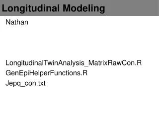
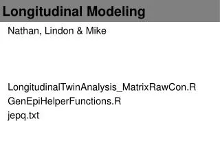
Longitudinal Modeling Nathan & Lindon Template_Developmental_Twin_Continuous_Matrix.R Template_Developmental_Twin_Ordinal_Matrix.R jepq.txt GenEpiHelperFunctions.R
Why run longitudinal models? Map changes in the magnitude of genetic & environmental influence across time ID same versus different genetic or environmental risks across development ID factors driving change versus factors maintaining stability Improve power to detect A, C & E - using multiple observations from the same individual & the cross twin cross trait correlations
Common methods for longitudinal data analyses in genetic epidemiology • Cholesky Decomposition • - Advantages • - Logical: organized such that all factors are constrained to impact later, but not earlier time points • - Requires few assumptions, can predict any pattern of change • - Disadvantages • - Not falsifiable • - No predictions • - Feasible for limited number of measurements • Latent Growth Curve Modeling • Simplex Modeling
Layout Recap Common Pathway Model Latent Growth Models Simplex Models A caveat emptor or two from Lindon
Phenotype 1 Phenotype 3 Phenotype 2 1 1 1 1 1 1 1 1 1 1 1 1 EC AC CC Common Pathway c11 a11 e11 Common Path f21 f11 f21 AS3 CS3 AS1 CS1 AS2 CS2 ES3 ES1 ES2
Phenotype 1 Phenotype 2 Phenotype 3 1 1 1 1 # Specify a, c & e path coefficients from latent factors A, C & E to Common Pathway mxMatrix( type="Lower", nrow=nf, ncol=nf, free=TRUE, values=.6, name="a" ), # Specify a, c & e path coefficients from residual latent factors As, Cs & Es to observed variables i.e. specifics mxMatrix( type="Diag", nrow=nv, ncol=nv, free=TRUE, values=4, name="as" ), # Specify factor loadings ‘f’ from Common Path to observed variables mxMatrix( type="Full", nrow=nv, ncol=nf, free=TRUE, values=15, name="f" ), # Matrices A, C, & E to compute variance components mxAlgebra( expression = f %&% (a %*% t(a)) + as %*% t(as), name="A" ), AC Common Pathway: Genetic components of variance a11 Common Path ’ as11 as11 ’ = A X as22 + as22 X & f21 as33 as33 f11 f21 as11 as22 as33 As3 As1 As2
# Matrices to store a, c, and e path coefficients for latent phenotype(s) mxMatrix( type="Lower", nrow=nf, ncol=nf, free=TRUE, values=.6, name="a" ), mxMatrix( type="Lower", nrow=nf, ncol=nf, free=TRUE, values=.6, name="c" ), mxMatrix( type="Lower", nrow=nf, ncol=nf, free=TRUE, values=.6, name="e" ), # Matrices to store a, c, and e path coefficients for specific factors mxMatrix( type="Diag", nrow=nv, ncol=nv, free=TRUE, values=4, name="as" ), mxMatrix( type="Diag", nrow=nv, ncol=nv, free=TRUE, values=4, name="cs" ), mxMatrix( type="Diag", nrow=nv, ncol=nv, free=TRUE, values=4, name="es" ), # Matrix f for factor loadings from common pathway to observerd phenotypes mxMatrix( type="Full", nrow=nv, ncol=nf, free=TRUE, values=15, name="f" ), # Matrices A, C, & E to compute variance components mxAlgebra( expression = f %&% (a %*% t(a)) + as %*% t(as), name="A" ), mxAlgebra( expression = f %&% (c %*% t(c)) + cs %*% t(cs), name="C" ), mxAlgebra( expression = f %&% (e %*% t(e)) + es %*% t(es), name="E" ), Common Pathway: Matrix algebra + variance components Within twin (co)variance
# Algebra for expected variance/covariance covMZ <- mxAlgebra( expression= rbind( cbind( A+C+E,A+C), cbind( A+C , A+C+E)), name="expCovMZ" ) covMZ <- mxAlgebra( expression= rbind( cbind( A+C+E , 0.5%x%A+C), cbind(0.5%x%A+C , A+C+E)), name="expCovMZ" ) CP Model: Expected covariance 1 1 / 0.5 Twin 1 Twin 2
Do means & variance components change over time? - Are G & E risks stable? How to best explain change? - Linear, non-linear? One solution == Latent Growth Model Build LGC from scratch Got longitudinal data? Phenotype 1 Time 1 Phenotype 1 Time 2 Phenotype 1 Time 3
AI EI CI 1 1 1 1 1 1 1 1 1 1 1 1 e11 c11 Common Pathway Model a11 B m f31 f11 f21 as33 as11 as22 es22 es11 es33 cs11 cs33 cs22 AS3 CS3 AS1 CS1 AS2 CS2 ES3 ES1 ES2
E1 A1 E2 C2 A2 C1 nf <- 1 nf <- 2 1 1 1 1 1 1 1 1 1 1 1 1 1 1 1 e11 c11 e22 CPM to Latent Growth Curve Model a11 a22 c22 B1 B2 m2 m1 f31 f12 f32 f22 f21 f11 Phenotype 1 Time 1 Phenotype 1 Time 2 Phenotype 1 Time 3 as33 as11 as22 es22 es11 es33 cs11 cs33 cs22 AS3 CS3 AS1 CS1 AS2 CS2 ES3 ES1 ES2
C1 E1 A1 A2 C2 E2 e21 c21 a21 nf <- 1 nf <- 2 1 1 1 1 1 1 1 1 1 1 1 1 1 1 1 e11 c11 e22 CP to Latent Growth Curve Model a11 a22 c22 B1 B2 m1 m2 f31 f12 f32 f22 f21 f11 Phenotype 1 Time 1 Phenotype 1 Time 2 Phenotype 1 Time 3 as33 as11 as22 es22 es11 es33 cs11 cs33 cs22 AS3 CS3 AS1 CS1 AS2 CS2 ES3 ES1 ES2
CI Es AI Cs As EI 1 1 1 1 1 1 1 1 1 1 1 1 1 1 1 Intercept: Factor which explains initial variance components (and mean) for all measures. Accounts for the stability over time. Slope: Factor which influences the rate of change in the variance components (and mean) over time. Slope(s) is (are) pre-defined: linear & non linear (quadratic, logistic, gompertz etc) hence factor loading constraints required. e11 c11 e22 Latent Growth Curve Model a11 a22 c22 e21 c21 a21 Bi Bs Intercept Slope im sm 1 0 2 1 1 1 Phenotype 1 Time 1 Phenotype 1 Time 2 Phenotype 1 Time 3 Twin 1 as33 as11 as22 es22 es11 es33 cs11 cs33 cs22 AS3 CS3 AS1 CS1 AS2 CS2 ES3 ES1 ES2
As AI 1 1 1 1 1 Genetic pathway coefficients matrix LGC Model: Within twin genetic components of variance a11 a22 a21 Intercept Slope 1 0 2 Factor loading matrix 1 1 1 Phenotype 1 Time 1 Phenotype 1 Time 2 Phenotype 1 Time 3 Twin 1 as33 as11 as22 aS11 Residual genetic pathway coefficients matrix aS22 AS3 AS1 AS2 aS33
# Matrix for a path coefficients from latent factors to Int’ & Slope latent factors pathAl <- mxMatrix( type="Lower", nrow=nf, ncol=nf, free=TRUE, values=.6, labels=AlLabs, name="al" ) # Matrix for a path coefficients from residuals to observed phenotypes pathAs <- mxMatrix( type="Diag", nrow=nv, ncol=nv, free=TRUE, values=4, labels=AsLabs, name="as" ) # Factor loading matrix of Int & Slop on observed phenotypes pathFl <- mxMatrix( type="Full", nrow=nv, ncol=nf, free=FALSE, values=c(1,1,1,0,1,2), name="fl" ) LGC Model: Specifying variance components in R ’ ’ aS11 aS11 = A aS22 aS22 X + & X aS33 aS33 # Matrix A to compute additive genetic variance components covA <- mxAlgebra( expression=fl %&% (al %*% t(al)) + as %*% t(as), name=“A”)
Simplex Models Simplex designs model changes in the latent factor structure over time by fitting auto-regressive or Markovian chains Determine how much variation in a trait is caused by stable & enduring effects versus transient effects unique to each time The chief advantage of this model is the ability to partition environmental & genetic variation at each time point into: - genetic & environmental effects unique to each occasion - genetic and environmental effects transmitted from previous time points
Simplex Models 1 1 1 1 1 1 I3 innovations I1 I2 i33 i11 i22 latent factor means latent factors LF1 LF3 LF2 lf32 lf21 means 1 1 1 m3 m2 m1 b3 b2 b1 Phenotype 1 Time 1 Phenotype 1 Time 2 Phenotype 1 Time 3 observed phenotype u33 u11 u22 measurement error me me me
Simplex Models: Within twin genetic variance A1 A2 A3 A1 Transmission pathways A2 A3 Innovation pathways
Simplex Models: Genetic variance A1 A2 A3 A1 Transmission pathways A2 A3 Innovation pathways -1 ’ & - = A * matI <- mxMatrix( type="Iden", nrow=nv, ncol=nv, name="I”) pathAt <- mxMatrix( type="Lower", nrow=nv, ncol=nv, free=tFree, values=ValsA, labels=AtLabs, name="at" ) pathAi <- mxMatrix( type="Diag", nrow=nv, ncol=nv, free=TRUE, values=iVals, labels=AiLabs, name="ai" ) covA <- mxAlgebra( expression=solve( I - at ) %&% ( ai %*% t(ai)), name="A" )
Simplex Models: E variance + measurement error matI <- mxMatrix( type="Iden", nrow=nv, ncol=nv, name="I”) pathEt <- mxMatrix( type="Lower", nrow=nv, ncol=nv, free=tFree, values=tValsE, labels=EtLabs, name="et" ) pathEi <- mxMatrix( type="Diag", nrow=nv, ncol=nv, free=TRUE, values=iVals, labels=EiLabs, name="ei" ) pathMe <- mxMatrix( type="Diag", nrow=nv, ncol=nv, free=TRUE, labels=c("u","u","u"), values=5, name="me" ) covE <- mxAlgebra( expression=solve( I-et ) %&% (ei %*% t(ei))+ (me %*% t(me)), name="E" ) ~ ’ & - * + ’ = E *
Ordinal Data Latent Growth Curve Modeling Es Cs As EI CI AI 1 1 1 1 1 1 1 1 1 1 1 1 1 1 1 e11 c11 e22 a11 a22 c22 e21 c21 a21 Bi Bs Intercept Slope im sm 1 0 2 1 1 1 Phenotype 1 Time 1 Phenotype 1 Time 2 Phenotype 1 Time 3 as33 as11 as22 es22 es11 es33 cs11 cs33 cs22 AS3 CS3 AS1 CS1 AS2 CS2 ES3 ES1 ES2
Ordinal Data Latent Growth Curve Modeling Two tasks: Estimate means Fix thresholds Assumes Measurement Invariance
Intercept Slope Im Sm 1 0 2 1 1 1 Phenotype 1 Time 1 Phenotype 1 Time 2 Phenotype 1 Time 3 Means on observed phenotypes versus means on Intercept & Slope? Bi Bs LGC Model: Estimating means (& sex) in R Twin 1 MeansIS<- mxMatrix( type="Full", nrow=2, ncol=1, free=T, labels=c("Im","Sm"), values=c(5,2), name="LMeans" ) pathB <- mxMatrix( type="Full", nrow=2, ncol=1, free=T, values=c(5,2), labels=c("Bi","Bs"), name="Beta" ) pathFl <- mxMatrix( type="Full", nrow=nv, ncol=nf, free=FALSE, values=c(1,1,1,0,1,2), labels=FlLabs,name="fl" ) # Read in covariates defSex1 <- mxMatrix( type="Full", nrow=1, ncol=1, free=FALSE, labels=c("data.sex_1"), name="Sex1")
Intercept Slope Im Sm 1 0 2 1 1 1 Phenotype 1 Time 1 Phenotype 1 Time 2 Phenotype 1 Time 3 + @ = Expected means for Twin 1 X LGC Model: Means Algebra = X Means1 <- mxAlgebra( expression= ( t((fl %*% ( LMeans - Sex1 %x% Beta )))), name="Mean1") Bi Bs Twin 1