Download
1 / 28
280 likes | 486 Views
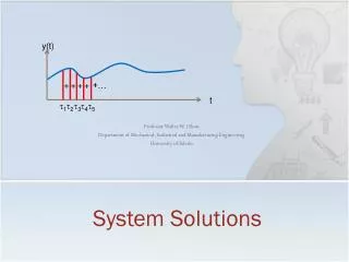
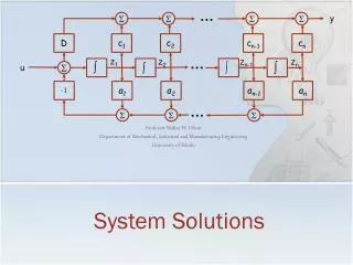
System Solutions. Professor Walter W. Olson Department of Mechanical, Industrial and Manufacturing Engineering University of Toledo. …. y. S. S. S. S. D. c 1. c 2. c n-1. c n. …. z 1. z 2. z n. z n-1. u. S. -1. a 1. a 2. a n-1. a n. …. S. S. S.

E N D
System Solutions Professor Walter W. Olson Department of Mechanical, Industrial and Manufacturing Engineering University of Toledo … y S S S S D c1 c2 cn-1 cn … z1 z2 zn zn-1 u S -1 a1 a2 an-1 an … S S S
Outline of Today’s Lecture • Review • Convolution Equation • Impulse Response • Step Response • Frequency Response • Linearization • Reachability • Testing for Reachability
Transformations • We can transform our state space representation to other state variables (different that the ones in use). • Mathematically, this is called a change of basis vectors. • Why would we ant to do this? • To make the problem easier to solve! • To isolate a particular property of the system • To uncouple the modes of the system
Transformations • Say we have some matrix T that is invertible (this is important) which results in the vector z when x is premultiplied by T. We then say that we have transformed the vector x into z, or alternatively, we have transformed x into z:
Convolution Equation is called the “Convolution Equation” Expresses the effect of an input on the system • What is convolution? • a twisting or folding together of two things • A convolution is found in many phenomena: • A sound that bounces off of a wall and interacts with the source sound is a convolution • A shadow is a convolution between the light source and the object producing the shadow • In statistics, a moving average is a convolution
The Impulse Function • Imagine a function that has a shape that is infinitesimally thin in the independent variable but infinitely high domain or response: • In other words this is a very long and sharp spike • This is what we try to model with the impulse function • Mathematically we define the Dirac Delta Function, d(t), also called the Impulse Function by
System Response Since our system is linear and we can add solutions, we can approximate the response as a sum of the convolutions of h(t-t)d(t) y(t) + + + + +… t t1 t2 t3 t4 t5
System Response S(t) • A unit step is defined as • With zero initial conditions 1 { Overshoot Mp t Steady State Rise time, tr Transient period=settling time, ts } } Transient Steady State
System Response • Another common test function is a sinusoid for frequency response • Since we have a linear system, we only need and assuming that the eigenvalues A do not equal s } } Steady State Transient
System Response: Frequency Response • Time history with respect to a sinusoid: Phase Shift, DT Amplitude Ay Amplitude Au Input Sin(t) Period,T Transient Response
System ResponseFrequency Response M is the magnitude and q is the phase
Linearization • Good solutions for the Linear Model • Equally good techniques for the Nonlinear Model are not easy to come by • What if the Nonlinear Model is well enough behaved in the region of interest so that we could apply Linear techniques strictly to that region? • We did this with the inverted pendulum! • We assumed small angles!
Linearization Techniques • Ignore the nonlinearity • In some cases, the nonlinearity has a relatively small effect • In those cases, build a linear system and treat the nonlinearity as a disturbance • Small angle approximations • Often only useful near equilibrium points • Taylor Series Truncation about an operating point • Assumes that 2nd and higher orders are negligible • Feedback linearization 0
Reachability • Consider the following problem: • With the linkage below, can you control the position of p? y’ yp y u(t) p x’ x
Reachability • We define reachability (often times called controllability) by the following: • A state in a system is reachable if for any valid states of the system, say, initial state at time t=0, x0 , and a state xf, there exists a solution for t>0 such that x(0) = x0 and x(t)=xf. • There are systems which we can not control • the states are not reachable with our input. • There in designing control systems, it is important to know if the system is controllable. • This is closely linked with the concept of ergodicity of the system in which we ask the question whether or not it is possible to with some measure of our system to measure every possible state of the system.
Reachability • For the system, , all of the states of the system are reachable if and only if Wr is invertible where Wr is given by
State Space Formulation • Is this a reachable system?
Example • Since the inverse of the reachability matrix exists, the system is reachable and controllable.
Matlab • Matlab has the function ctrb(A,B) which will compute the reachability matrix: >> Wr=ctrb(A,B) Wr = 1.0e+014 * 0 0 0.0000 -0.0000 0 0.0000 -0.0000 0.0000 0 0.0000 -0.0000 0.0016 0.0000 -0.0000 0.0016 -3.8688 >> inv(Wr) Warning: Matrix is close to singular or badly scaled. Results may be inaccurate. RCOND = 9.669679e-017. ans = 0.9937 23.7500 -0.4938 0.0000 23.7500 -10.0000 0.2500 0 1.9750 -0.9992 0.0250 0 0.0008 -0.0004 0.0000 0 >> A=[0 1 0 0; -0.05 -0.025 0.05 0.025;... 0 0 0 1; 5000 2500 -30000 -2500] A = 1.0e+004 * 0 0.0001 0 0 -0.0000 -0.0000 0.0000 0.0000 0 0 0 0.0001 0.5000 0.2500 -3.0000 -0.2500 >> B = [0;0;0;25000] B = 0 0 0 25000
Canonical Forms • The word “canonical” means prescribed • In Control Theory there a number transformations that can be made to put a system into a certain canonical form where the structure of the system is readily recognized • One such form is the Controllable or Reachable Canonical form.
Reachable Canonical Form • A system is in the reachable canonical form if it has the structure Such a structure can be represented by blocks as … y S S S S D c1 c2 cn-1 cn … z1 z2 zn zn-1 u S -1 a1 a2 an-1 an … S S S
Reachable Canonical Form • It can be shown that the characteristic polynomial is • To convert to Reachable Canonical Form, consider the transformation
Example: Inverted Pendulum • Develop the reachability canonical form for the Segway using the inverted pendulum model of Lecture 5
Summary • Reachability • A state in a system is reachable if for any valid states of the system, say, initial state at time t=0, x0 , and a state xf, there exists a solution for t>0 such that x(0) = x0 and x(t)=xf. • Testing for Reachability • For the system, , all of the states of the system are reachable if and only if Wr is invertible where Wr is given by Next: State Feedback