Download

1 / 17
170 likes | 196 Views
This project utilizes finite-difference method to solve 2D steady state conduction problems in a square plate, providing approximate temperature solutions. It employs iterative process for temperature calculations.

E N D
Hot plate Conduction Numerical Solver and Visualizer Kurt Hinkle and Ivan Yorgason
Introduction • There are analytical methods that, in certain cases, can produce exact mathematical solutions to 2D steady state conduction problems. • There are even solutions that are available for simple geometries with specific boundary conditions that can be used simply by plugging in numbers. • Sometimes, however, there are geometries and/or boundary conditions that are not covered by the aforementioned solutions. • When this occurs, numerical techniques, such as finite-difference, finite-element, and boundary-element methods are used to provide approximate solutions. • This project uses the finite-difference form of the heat equation to solve for the temperatures across a square plate.
Limitations and assumptions • 2D steady state conduction • Constant wall temperatures • No convection • Square plate • Square elements • Temperatures ranging 0ºC - 1000ºC • Mesh size ranging 3 - 80
Method Mesh
500ºC 500ºC 500ºC Method Initial Values 1000ºC 0ºC 0ºC 0ºC 0ºC 0ºC 0ºC 1000ºC 0ºC 0ºC 1000ºC 0ºC 0ºC 0ºC 0ºC 100ºC 100ºC 100ºC
500ºC 500ºC 500ºC Method 1000ºC 375ºC 0ºC 0ºC ? 0ºC Calculate First Element Temperature (1000ºC + 500ºC + 0ºC + 0ºC)/4 = 375ºC 0ºC 0ºC 1000ºC 0ºC 0ºC 1000ºC 0ºC 0ºC 0ºC 0ºC 100ºC 100ºC 100ºC
500ºC 500ºC 500ºC Method 1000ºC 375ºC 218.8ºC 0ºC 179.7ºC 1st Iteration Complete 343.8ºC 140.6ºC 1000ºC 80.1ºC 0ºC 1000ºC 360.9ºC 150.4ºC 0ºC 82.6ºC 100ºC 100ºC 100ºC
500ºC 500ºC 500ºC Method 1000ºC 515.6ºC 333.9ºC 0ºC 228.5ºC 2nd Iteration Complete 504.3ºC 267.2ºC 1000ºC 144.6ºC 0ºC 1000ºC 438.7ºC 222.1ºC 0ºC 116.7ºC 100ºC 100ºC 100ºC
500ºC 500ºC 500ºC Method 1000ºC 584.6ºC 395.1ºC 0ºC 259.9ºC 3rd Iteration Complete 572.6ºC 333.6ºC 1000ºC 177.5ºC 0ºC 1000ºC 473.7ºC 255.9ºC 0ºC 133.4ºC 100ºC 100ºC 100ºC
Method • Differences with finite-difference method • Instead of setting up a matrix and inverting it to solve for all temperatures at once, the temperatures are solved for through an iterative process. • This iterative process (N^2 algorithm) is limited by a time which is calculated based on the mesh size. Larger mesh sizes are allowed more time to iteratively solve for the element temperatures.
Functionality Temperature: The temperature of the wall. Mesh Size: The number of elements between opposite walls. Calculate: Calculates the element temperatures and displays them colorfully. Print: Calculates the element temperatures and once the algorithm is complete, it prints the resulting element temperatures to results.dat in a matrix format along with the wall temperatures. Close: Closes the program.
Functionality • Live Demo: • 14.exe
Future Work • Allow for other shapes and holes in the geometry • Allow for different mesh element types (tetrahedral, etc.) • Stop the iterative solver based on a tolerance instead of a time limit • Export .jpg of visualized results with results.dat file • Have the color scheme be relative to the maximum and minimum temperatures instead of the scale being absolute (1000ºC = red and 0ºC = blue).
Conclusion • Provides quick and accurate results for the given assumptions • Graphically displays the results in an understandable and pleasing manner • With the option to print the results to a file, further analysis is easily accomplished • The finite-difference form of the heat equation is easy to implement programmatically