Download
1 / 26
260 likes | 456 Views
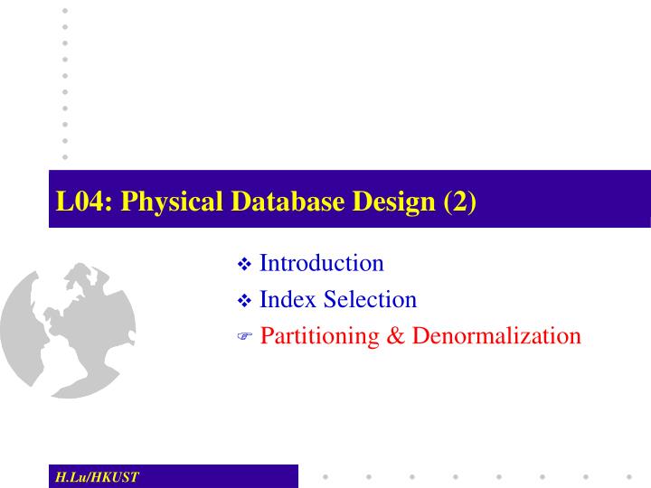
L04: Physical Database Design (2). Introduction Index Selection Partitioning & Denormalization. Tuning a Relational Schema. The choice of relational schema should be guided by the workload, in addition to redundancy issues: We may settle for a 3NF schema rather than BCNF.

E N D
L04: Physical Database Design (2) Introduction Index Selection Partitioning & Denormalization
Tuning a Relational Schema • The choice of relational schema should be guided by the workload, in addition to redundancy issues: • We may settle for a 3NF schema rather than BCNF. • Workload may influence the choice we make in decomposing a relation into 3NF or BCNF. • We might denormalize(i.e., undo a decomposition step), or we might add fields to a relation • We may further decompose a BCNF schema! • We might consider horizontal partitioning. • If such changes are made after a database is in use, called schema evolution; might want to mask some of these changes from applications by defining views.
Example Schemas Contracts (Cid, Sid, Jid, Did, Pid, Qty, Val) Depts (Did, Budget, Report) Suppliers (Sid, Address) Parts (Pid, Cost) Projects (Jid, Mgr) • We will concentrate on Contracts, denoted as CSJDPQV. The following ICs are given to hold: JPC, SD P, Cis the primary key. • What are the candidate keys for CSJDPQV? • What normal form is this relation schema in?
Denormalization • Suppose that the following query is important: • Is the value of a contract less than the budget of the department? • To speed up this query, we might add a field budget B to Contracts. • This introduces the FD DB wrt Contracts. • Thus, Contracts is no longer in 3NF. • We might choose to modify Contracts thus if the query is sufficiently important, and we cannot obtain adequate performance otherwise (i.e., by adding indexes or by choosing an alternative 3NF schema.)
Partitioning • Horizontal Partitioning: Distributing the rows of a table into several separate files • Useful for situations where different users need access to different rows • Vertical Partitioning: Distributing the columns of a table into several separate files • Useful for situations where different users need access to different columns • The primary key must be repeated in each file • Combinations of Horizontal and Vertical Partitions often correspond with User Schemas (user views)
Partitioning • Advantages of Partitioning: • Records used together are grouped together • Each partition can be optimized for performance • Security, recovery • Partitions stored on different disks: contention • Take advantage of parallel processing capability • Disadvantages of Partitioning: • Slow retrievals across partitions • Complexity • Issues: Need to find suitable level • Too little too much of irrelevant data access. • Too much too much processing cost
Horizontal Decompositions • Our definition of decomposition: Relation is replaced by a collection of relations that are projections. Most important case. • Sometimes, might want to replace relation by a collection of relations that are selections. • Each new relation has same schema as the original, but a subset of the rows. • Collectively, new relations contain all rows of the original. Typically, the new relations are disjoint.
Horizontal Decompositions (Contd.) • Suppose that contracts with value > 10000 are subject to different rules. This means that queries on Contracts will often contain the condition val>10000. • One way to deal with this is to build a clustered B+ tree index on the val field of Contracts. • A second approach is to replace contracts by two new relations: LargeContracts and SmallContracts, with the same attributes (CSJDPQV). • Performs like index on such queries, but no index overhead. • Can build clustered indexes on other attributes, in addition!
Masking Conceptual Schema Changes CREATE VIEW Contracts(cid, sid, jid, did, pid, qty, val) AS SELECT * FROM LargeContracts UNION SELECT * FROM SmallContracts • The replacement of Contracts by LargeContracts and SmallContracts can be masked by the view. • However, queries with the condition val>10000 must be asked wrt LargeContracts for efficient execution: so users concerned with performance have to be aware of the change.
Decomposition of a BCNF Relation • Suppose that we choose { SDP, CSJDQV }. This is in BCNF, and there is no reason to decompose further (assuming that all known ICs are FDs). • However, suppose that these queries are important: • Find the contracts held by supplier S. • Find the contracts that department D is involved in. • Decomposing CSJDQV further into CS, CD and CJQV could speed up these queries. (Why?) • On the other hand, the following query is slower: • Find the total value of all contracts held by supplier S.
Vertical Partitioning • Vertical partitioning of a relation R produces partitions R1, R2, ..., Rm, each of which contains a subset of R's attributes as well as the primary key of R • The object of vertical partitioning is to reduce irrelevant attribute access, and thus irrelevant data access • ``Optimal'' vertical partitioning minimizes the irrelevant data access for user applications • For a relation with m non-primary key attributes, the number of possible partitions is approximately equal to mm • Hard to find an optimal solution • Resort to heuristic approaches
VP: Heuristic Approaches • Grouping: • Assign each attribute to one fragment • Join fragments until some criteria is satisfied • Splitting (our focus): • Start with the original relation • Generate partitions based on access behavior • Closer to optimal; less overlapping fragments • Basic idea: Affinity of attributes • A measure of closeness of these attributes
Attribute Usage Matrices • Q = {q1 , q2, ..., qm} • Set of user queries • R (A1, A2, ..., An) • Relation R with n attributes • Usage matrix |Uij|m×n • Uij = 1 if attribute Aj is referenced by qi; • Uij = 0 otherwise. • Access matrix |acci| • access frequency of qi
VP - Matrices Examples • Relation PROJ(PNO,PNAME,BUDGET,LOC), four SQL queries sent to three sites: q1: SELECT BUDGET FROM PROJ WHERE PNO = val; q2: SELECT PNAME,BUDGET FROM PROJ; q3: SELECT PNAME FROM PROJWHERE LOC = val; q4: SELECT SUM(BUDGET) FROM PROJ WHERE LOC=val;
Attribute Affinity Matrix • |affij|n×n : Affinity between two attributes Ai and Aj affij = { k|Uki = 1 Ukj =1} acck AA Matrix
Bond Energy Clustering Algorithm • Determines groups of similar items (clusters of attributes with larger affinity values, and ones with smaller affinity values) • Final groupings are insensitive to the order in which items are presented to the algorithm • The computation time is O(n2 ) where n is the number of attributes • Secondary interrelationships between clustered attribute groups are identifiable
Main Idea of BEA Permute the attribute affinity matrix (AA) and generate a clustered affinity matrix (CA) to maximize the global affinity measure (AM) where
AM in Terms of Bond Because the affinity matrix is symmetric, , or Let then AM = ∑[bond(Aj, Aj-1) + bond(Aj, Aj+1)]
Bond Energy Algorithm • Initialization : place and fix one of the columns of AA arbitrarily into CA • Iteration : • Pick one of the remaining ni columns of AA and place it in one of the i+1 positions in CA • Choose the placement that makes greatest contribution. • Row ordering : • Change the placement of the rows accordingly
Contribution of a Placement Contribution of placing attribute Akbetween Ai and Aj : cont(Ai, Ak, Aj) = 2bond(Ai, Ak) + 2bond(Ak, Aj) – 2bond(Ai, Aj) bond(A1, A2) = 45*0+0*80+45*5+0*75=225 bond(A1, A4) = 45*0+0*75+45*3+0*78=135 bond(A4, A2) = 0*0+ 75*80+3*5+78*75=11865 If we place A4between A1 and A2, cont(A1, A4, A2 ) = 2bond(A1, A4) + 2bond(A4, A2) – 2bond(A1, A2) = 2*135 + 2*11865 - 2*225 = 23550
A1A3 A2 A4 A1A3 A2 A4 BEA Example A1A3 A2 A3 A1A2 A1A2 A3 A4 A1A2 A3 A4 A1A3 A2 A4 A1A2 A3 A4 cont(A0, A3, A1)= 8820 cont(A1, A3, A2)= 10150 cont(A2, A3, A4)= 1780 Two clusters: the upper left corner of the smaller affinity values, and the lower right corner of the larger affinity values
A1A2A3 … Ai Ai+1 An A1A2A3 . Ai Ai+1 An TA BA VP Splitting The basic idea Given a set of attributes {A1, A2, ..., An} and a set of applications, partition the attributes into two or more sets such that there are no (or minimal) applications that access more than one of the sets. Two attribute sets: TA : {A1, A2, ..., Ai} BA : {Ai+1, Ai+2, ..., An} TQ Three sets of apps: TQ : access TA only BQ : access BAonly OQ: access both OQ BQ
VP Splitting Problem Define: • CTQ = total number of accesses to attributes by applications that access only TA • CBQ = total number of accesses to attributes by applications that access only BA • COQ = total number of accesses to attributes by applications that access both TA & BA Find a split point x (1≤x<n) which maximizes z z = CTQ * CBQ COQ2
VP – The Splitting Algorithm • Input: Relation R, and CA, acc matrices • Output: a set of fragments • For each split point x (1≤x<n) , compute z • Choose the split point with the maximum z value and construct fragments XQ {TQ, BQ, OQ}
TA BA TQ BQ OQ CTQ CBQ COQ z A1A3 A2 A4 A1 A3,2,4 Q2,3,4 Q1 0 83 45 -2025 A1A3 A2 A4 A1,3 A2,4 Q1 Q3 Q2,4 45 75 8 3311 A1,3,2 A4 Q1,2 Q3,4 50 0 78 -6084 VP: Splitting Example x 1 2 3 Partition: (A1,A3) (A2,A4)
Complications in VP Partitioning Algorithm • Cluster forming in the middle of the CA matrix • Shift a row up and a column left and apply the algorithm to find the “best” partitioning point • Do this for all possible shifts • Cost O(n2) • More than two clusters • M-way partitioning • Try 1, 2, …, m-1 split points along the diagonal and try to find the best point for each of these • Cost O(2m)