Download
1 / 31
320 likes | 698 Views
Spectral Leakage in the Discrete Fourier Transform. Greg Adams, LMCO MS2, 4/10/07.

E N D
Spectral Leakage in the Discrete Fourier Transform Greg Adams, LMCO MS2, 4/10/07
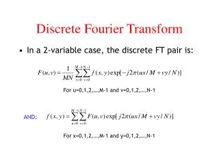
Synchronous Sampling is typically used with a Discrete Fourier Transform when testing analog to digital converters in the laboratory. A pure sine wave test signal is generated at such a frequency that the input signal goes through a whole number of cycles during the sampling period. If the test signal is slightly off frequency, i.e. the input signal doesn’t complete a whole number of cycles within the DFT time window, A distortion called spectral leakage occurs. A small frequency error has little effect on the main signal, but has a strong effect on the DFT noise floor. The relationship between frequency error, and the signal to noise ratio due to leakage noise has been established. This relationship can be used to determine the frequency resolution which the sine wave generator must have in order to generate a sine wave at a sufficiently accurate frequency. A simple calculator program is provided to evaluate the equations. Spectral Leakage in the Discrete Fourier Transform LMCO NE&SS SS Math & Physics Seminar 16 April 2003 Greg Adams, 856 722 4705 http://www.motown.lmco.com/~gadams/
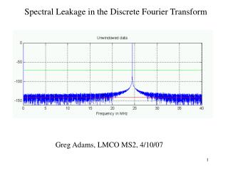
FFT, On Frequency fs=80e6, N=32768, signal freq = 24 MHz, FFT Bin size = 2441 Hz
Time Discontinuity One way of looking at the leakage problem is to observe the requirement that the Fourier Series operate on a periodic data set. If the off-frequency sinusoid is repeated to generate a periodic signal as shown, there is a discontinuity in the waveform. The resulting signal is not sinusoidal.
The Fourier Series (1) Where: The Fourier Series may be used to express any periodic function of TIME as the sum of Sine and Cosine functions of TIME. (expressed here in complex exponential form) Note that the coefficients Cn are derived by Correlating f(t) with the Discrete frequency sinusoids sin(nt) and cos(nt). The condition that f(t) be Periodic insures that it can be represented as a sum of Discrete sine and cosine functions. (whether Laurent believed it or not! )
The Fourier Series (2) A Fourier series may be used, for example, to show that a square wave is the sum of a sine wave, and all of it’s odd harmonics.
The Fourier Series (3) While the independent variable may be something other than time, and the Series may break the function down in terms of any complete set of Orthogonal functions, this discussion will assume a function of time, Broken down into a sum of circular functions (of time). We’ll also be restricting ourselves to real-valued functions of time.
The Fourier Transform The Fourier Transform is an extension of the Fourier Series. Whereas the Fourier Series was restricted to periodic functions of (t), the Transform may be applied functions which are aperiodic. While the Fourier SERIES resulted in an infinite series of discrete frequencies, the TRANSFORM, F(w) is a continuous function of frequency, defined for all real values of frequency. A continuous function of frequency
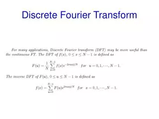
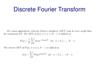
The Discrete Fourier Transform The Discrete Fourier Transform transforms a Finite length series of Discrete time samples f(k), into a Finite length, series of Discrete frequency samples F(n).
Finite Length Because the DFT operates on a data set of finite length, the Function f(t) must be multiplied by a rectangular window function before Being transformed. The window function is defined to be One for –p < t < p, and zero otherwise. This is the first function Appearing in our table of transforms, with T=2p. We’ll denote this window function as B(t) since it’s sometimes called a Boxcar Window*. *AKA the gate function, or the rectangular function.
Discrete time samples Because the DFT must operate on a data set consisting of discrete time samples, the Function f(t) must also be multiplied by a Picket Fence function, P(t), defined as: This product B(t)*P(t)*f(t) is the input data set on which our DFT will operate.
Series, Transform, DFT compared Fourier Series Coefficients DFT Fourier Transform • By comparing the defining equations, we can see that the DFT is proportional to the set of Fourier Series coefficients of B(t)*P(t)*f(t), with the substitution: • The DFT is integrated (summed) over an interval equivalent to 0 to 2p, while the Fourier Series is integrated over –p to p. • The terms of the DFT are equal to the integrand of the Fourier Transform of B(t)*P(t)*f(t), with the additional substitution.
Table of Properties From the table above, we see that the DFT has more in common with the Fourier Series than the Transform. The DFT and the Fourier Series both have a finite time interval of integration, and therefore yield discrete frequency samples. The DFT alone uses discrete time samples, and is therefore limited to a finite frequency interval as well.
Equivalence of DFT and Fourier Series Since the Fourier Series coefficients Cn were shown to be Proportional to the DFT frequency coefficients Fn, the RATIO of signal to integrated noise power will be identical whether we use the DFT or the series. We will proceed to quantify the ratio of Signal to Integrated Leakage Noise in a Fourier Series, having proved that this signal to noise ratio is the same whether we use the series or the DFT. The Integrated Leakage Noise is defined as the sum of the noise powers, at all frequencies other than the desired one, which result from the frequency error.
Notation The traditional notation used for the DFT is incompatible with the traditional notation used for the Fourier Series. We’ll be using the following harmonized notation: t= time, seconds f(t)= function of time, the input function N= Number of time samples used k= index of the k’th time sample n= Harmonic index, e.g. the n’th frequency bin. Cn=Coefficient of the n’th harmonic, Fourier Series Cs= Coefficient of the n’th sideband, Fourier Series F(n)=DFT of f(k) fa= analog signal frequency, Hz fs= sample rate, Hz m= number or whole sine waves sampled S= sideband number P= integrated noise power P(t)= ‘Picket fence’ function
The Riemann zeta function of p Notation (cont.) Fourier Transform of f(t) Radian Frequency Frequency Error, as a fraction of on frequency BIN Dirac's delta function B(t)= The Boxcar function (boxcar window)
Fourier Series, with frequency error Frequency Error, as a fraction of The frequency resolution. Sideband Number Sinusoid with frequency error Fourier Series expressed in terms of integer frequency m, plus error.
Evaluate the integral Integer frequency now expressed as “sideband number” S Indefinite integral evaluated
The arithmetic for small delta, and We now have an approximation to Cs, the noise amplitude in each sideband.
Summing the Sidebands The noise power in each sideband is proportional to Cs^2. There are infinitely many sidebands above and below the “carrier”. The sidebands which fall outside the normal frequency range alias back into the output spectrum, so we must sum Cs^2 for all S not zero, from positive to negative infinity. Since Cs^2=(-Cs)^2, we can Just sum from 1 to positive infinity, and multiply by two. But The above sum is equal to the Riemann Zeta function of 2, which Euler solved Explicitly in 1736.
Signal to Noise Ratio If some sidebands are to be omitted in the calculation of SNR, which is often the case, we may use the expression: For sidebands 1 through d removed In same units as
Testing the theory The Leakage Noise was estimated using the formula from the previous page, for a signal sampled at 80MSPS, with frequency offset errors ranging from 0.01 to 1000 Hz. The FFT frequency resolution will be 2441.40625 Hz. A sinusoid was generated by software. The resulting sine wave was truncated to 16 bit resolution. This signal’s frequency was varied over the same range of frequency offsets. An analog to digital converter was set up to sample a signal at 80 MSPS. The analog input signal frequency was adjusted over the same range of frequency offsets. A 32756 point FFT was performed on both the computer generated signal, and the signal sampled by the analog to digital converter. The resulting signal to noise ratios are tabulated below.
Results FFT Bin size = 2441 Hz, nearest three sidebands removed. fs=80e6, N=32768, signal freq = 24 MHz At .01 Hz error, the real data shows ADC thermal noise.
Results cont. The computer generated data had a signal to noise ratio of 97.08 dB. The noise on the signal results from truncating the data to 16 bits. The Analog to digital converter had a noise floor of 79.29 dB. The noise on this signal is thermal noise from the analog input circuit. When the leakage noise, as predicted in the first column, is well below the process noise, the FFT provides an accurate measure of process noise. When the leakage noise is significant compared with the process noise, the noise measured by the FFT is the sum of the process and leakage noise. The approximation may be used to determine what frequency accuracy is required, or how many sidebands must be discarded, to measure a given signal to noise ratio within a given error bound.