Download

1 / 75
750 likes | 936 Views
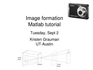
Image formation. Monday March 21 Prof. Kristen Grauman UT-Austin. Announcements. Reminder: Pset 3 due March 30 Midterms: pick up today. Recap: Features and filters. Transforming and describing images; textures, colors, edges. Kristen Grauman. Recap: Grouping & fitting.

E N D
Image formation Monday March 21 Prof. Kristen Grauman UT-Austin
Announcements • Reminder: Pset 3 due March 30 • Midterms: pick up today
Recap: Features and filters Transforming and describing images; textures, colors, edges Kristen Grauman
Recap: Grouping & fitting [fig from Shi et al] Clustering, segmentation, fitting; what parts belong together? Kristen Grauman
Multiple views Multi-view geometry, matching, invariant features, stereo vision Lowe Hartley and Zisserman Kristen Grauman
Plan • Today: • Local feature matching btwn views (wrap-up) • Image formation, geometry of a single view • Wednesday: Multiple views and epipolar geometry • Monday: Approaches for stereo correspondence
Previously Local invariant features • Detection of interest points • Harris corner detection • Scale invariant blob detection: LoG • Description of local patches • SIFT : Histograms of oriented gradients • Matching descriptors
Local features: main components • Detection: Identify the interest points • Description:Extract vector feature descriptor surrounding each interest point. • Matching: Determine correspondence between descriptors in two views Kristen Grauman
“flat”region “edge”: “corner”: Recall: Corners as distinctive interest points 1 >> 2 1 and 2 are small; 1 and 2 are large,1 ~ 2; 2 >> 1 One way to score the cornerness:
Harris Detector: Steps Compute corner response f
Blob detection in 2D: scale selection • Laplacian-of-Gaussian = “blob” detector filter scales img2 img1 img3
Blob detection in 2D • We define the characteristic scale as the scale that produces peak of Laplacian response characteristic scale Slide credit: Lana Lazebnik
Example Original image at ¾ the size Kristen Grauman
Scale invariant interest points Interest points are local maxima in both position and scale. s5 s4 scale s3 s2 List of(x, y, σ) s1 Squared filter response maps Kristen Grauman
Scale-space blob detector: Example T. Lindeberg. Feature detection with automatic scale selection. IJCV 1998.
Local features: main components • Detection: Identify the interest points • Description:Extract vector feature descriptor surrounding each interest point. • Matching: Determine correspondence between descriptors in two views Kristen Grauman
p 2 0 SIFT descriptor [Lowe 2004] • Use histograms to bin pixels within sub-patches according to their orientation. Why subpatches? Why does SIFT have some illumination invariance? Kristen Grauman
Making descriptor rotation invariant CSE 576: Computer Vision • Rotate patch according to its dominant gradient orientation • This puts the patches into a canonical orientation. Image from Matthew Brown
SIFT descriptor [Lowe 2004] • Extraordinarily robust matching technique • Can handle changes in viewpoint • Up to about 60 degree out of plane rotation • Can handle significant changes in illumination • Sometimes even day vs. night (below) • Fast and efficient—can run in real time • Lots of code available • http://people.csail.mit.edu/albert/ladypack/wiki/index.php/Known_implementations_of_SIFT Steve Seitz
SIFT properties • Invariant to • Scale • Rotation • Partially invariant to • Illumination changes • Camera viewpoint • Occlusion, clutter
Local features: main components • Detection: Identify the interest points • Description:Extract vector feature descriptor surrounding each interest point. • Matching: Determine correspondence between descriptors in two views Kristen Grauman
Matching local features Kristen Grauman
Matching local features ? Image 2 Image 1 To generate candidate matches, find patches that have the most similar appearance (e.g., lowest SSD) Simplest approach: compare them all, take the closest (or closest k, or within a thresholded distance) Kristen Grauman
Ambiguous matches ? ? ? ? Image 2 Image 1 At what SSD value do we have a good match? To add robustness to matching, can consider ratio : distance to best match / distance to second best match If low, first match looks good. If high, could be ambiguous match. Kristen Grauman
Matching SIFT Descriptors • Nearest neighbor (Euclidean distance) • Threshold ratio of nearest to 2nd nearest descriptor Lowe IJCV 2004 Derek Hoiem
Recap: robust feature-based alignment Source: L. Lazebnik
Recap: robust feature-based alignment • Extract features Source: L. Lazebnik
Recap: robust feature-based alignment • Extract features • Compute putative matches Source: L. Lazebnik
Recap: robust feature-based alignment • Extract features • Compute putative matches • Loop: • Hypothesize transformation T (small group of putative matches that are related by T) Source: L. Lazebnik
Recap: robust feature-based alignment • Extract features • Compute putative matches • Loop: • Hypothesize transformation T (small group of putative matches that are related by T) • Verify transformation (search for other matches consistent with T) Source: L. Lazebnik
Recap: robust feature-based alignment • Extract features • Compute putative matches • Loop: • Hypothesize transformation T (small group of putative matches that are related by T) • Verify transformation (search for other matches consistent with T) Source: L. Lazebnik
Applications of local invariant features Wide baseline stereo Motion tracking Panoramas Mobile robot navigation 3D reconstruction Recognition …
Automatic mosaicing http://www.cs.ubc.ca/~mbrown/autostitch/autostitch.html
Wide baseline stereo [Image from T. Tuytelaars ECCV 2006 tutorial]
Recognition of specific objects, scenes Sivic and Zisserman, 2003 Schmid and Mohr 1997 Lowe 2002 Rothganger et al. 2003 Kristen Grauman
Plan • Today: • Local feature matching btwn views (wrap-up) • Image formation, geometry of a single view • Wednesday: Multiple views and epipolar geometry • Monday: Approaches for stereo correspondence
Image formation • How are objects in the world captured in an image?
Physical parameters of image formation • Geometric • Type of projection • Camera pose • Optical • Sensor’s lens type • focal length, field of view, aperture • Photometric • Type, direction, intensity of light reaching sensor • Surfaces’ reflectance properties
Image formation • Let’s design a camera • Idea 1: put a piece of film in front of an object • Do we get a reasonable image? Slide by Steve Seitz
Pinhole camera • Add a barrier to block off most of the rays • This reduces blurring • The opening is known as the aperture • How does this transform the image? Slide by Steve Seitz
Pinhole camera • Pinhole camera is a simple model to approximate imaging process, perspective projection. Image plane Virtual image pinhole If we treat pinhole as a point, only one ray from any given point can enter the camera. Fig from Forsyth and Ponce
Camera obscura In Latin, means ‘dark room’ "Reinerus Gemma-Frisius, observed an eclipse of the sun at Louvain on January 24, 1544, and later he used this illustration of the event in his book De Radio Astronomica et Geometrica, 1545. It is thought to be the first published illustration of a camera obscura..." Hammond, John H., The Camera Obscura, A Chronicle http://www.acmi.net.au/AIC/CAMERA_OBSCURA.html
Camera obscura Jetty at Margate England, 1898. An attraction in the late 19th century Around 1870s http://brightbytes.com/cosite/collection2.html Adapted from R. Duraiswami
Camera obscura at home http://blog.makezine.com/archive/2006/02/how_to_room_sized_camera_obscu.html Sketch from http://www.funsci.com/fun3_en/sky/sky.htm
Perspective effects • Far away objects appear smaller Forsyth and Ponce
Perspective effects • Parallel lines in the scene intersect in the image • Converge in image on horizon line Image plane (virtual) pinhole Scene