Download
1 / 8
80 likes | 421 Views
Chi square and Hardy-Weinberg. Problem #1. A study on blood types in a population found the following genotypic distribution among the people sampled: 1101 were MM, 1496 were MN 503 were NN

E N D
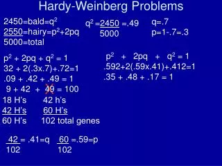
Problem #1 • A study on blood types in a population found the following genotypic distribution among the people sampled: • 1101 were MM, • 1496 were MN • 503 were NN • Calculate the allele frequencies of M and N, the expected numbers of the three genotypic classes (assuming random mating). • Using X2, determine whether or not this population is in Hardy-Weinberg equilibrium.
GENOTYPE FREQUENCIES: • MM (p2) = 1101/3100 = 0.356 • MN (2pq) = 1496/3100 = 0.482 • NN (q2) = 503/3100 = 0.162
ALLELE FREQUENCIES: • Freq of M • p = p2 + 1/2 (2pq) • 0.356 + 1/2 (0.482) = 0.356 + 0.241 = 0.597 • Freq of N • q = 1- p • 1 - 0.597 = 0.403. This is more accurate than taking the square root of q2
EXPECTED GENOTYPE FREQUENCIES (assuming Hardy-Weinberg): • MM (p2) = (0.597)2 = 0.357 • MN (2pq) = 2 (0.597)(0.403) = 0.481 • NN (q2) = (0.403)2 = 0.162
EXPECTED NUMBER OF INDIVIDUALS of EACH GENOTYPE: • # MM = 0.357 X 3100 = 1107 • # MN = 0.481 X 3100 = 1491 • # NN = 0.162 X 3100 = 502
CHI - SQUARE (X2): X2 = Σ(O - E)2 / E X2 = (1101-1107)2 /1107 + (1496-1491)2 /1491 + (502-503)2 /503 • = (-6)2 /1107 + (5)2 /1491 + (-1)2 /503 • = 0.0325 + 0.0168 + 0.002 • = 0.0513 • X2 (calculated) < X2 (table) [3.841, 1 df, 0.05 ].
Accept or Reject • Therefore, conclude that there is no statistically significant difference between what you observed and what you expected under Hardy-Weinberg. • Accept null hypothesis and conclude that the population is in HWE. • Population is not evolving