Download

1 / 36
410 likes | 963 Views
Bitmap Indexing. Bitmap Index. Bitmap index: specialized index that takes advantage Read-mostly data: data produced from scientific experiments can be appended in large groups Fast operations “Predicate queries” can be performed with bitwise logical operations

E N D
Bitmap Index • Bitmap index: specialized index that takes advantage • Read-mostly data: data produced from scientific experiments can be appended in large groups • Fast operations • “Predicate queries” can be performed with bitwise logical operations • Predicate ops: =, <, >, <=, >=, range, • Logical ops: AND, OR, XOR, NOT • They are well supported by hardware • Easy to compress, potentially small index size • Each individual bitmap is small and frequently used ones can be cached in memory
Bitmap Index • Can be useful for stable columns with few values • Bitmap: • String of bits: 0 (no match) or 1 (match) • One bit for each row • Bitmap index record • Column value • Bitmap • DBMS converts bit position into row identifier.
Bitmap Index Example Faculty Table Bitmap Index on FacRank
Compressing Bitmaps:Run Length Encoding • Bit vector for Assc: 0010000000010000100 • Runs: 2, 8, 4 • Can we do: 10 1000 100? Is this unambiguous? • Fixed bits per run (max=4) • 0010 1000 0100 • Variable bits per run • 1010 11101000 110100 • 11101000 is broken into: 1110 (#bits), 1000 (value) • i.e., 4 bits are required, value is 8
Operation-efficient Compression Methods Based on variations of Run Length Compression Uncompressed: 0000000000001111000000000 ......0000001000000001111111100000000 .... 0000100 Compressed: 12, 0, 0, 0, 0, 1000, 8, 0, 0, 0, 0, 0, 0, 0, 0, 1000 Store very short sequences as-is AND/OR/COUNT operations: Can uncompress on the fly
Indexing High-Dimensional Data • Typically, high-dimensional datasets are collections of points, not regions. • E.g., Feature vectors in multimedia applications. • Very sparse • Nearest neighbor queries are common. • R-tree becomes worse than sequential scan for most datasets with more than a dozen dimensions. • As dimensionality increases contrast (ratio of distances between nearest and farthest points) usually decreases; “nearest neighbor” is not meaningful. • In any given data set, advisable to empirically test contrast.
Why Sort? • A classic problem in computer science! • Data requested in sorted order • e.g., find students in increasing gpa order • Sorting is first step in bulk loading B+ tree index. • Sorting useful for eliminating duplicate copies in a collection of records (Why?) • Sort-merge join algorithm involves sorting. • Problem: sort 1Gb of data with 1Mb of RAM. • why not virtual memory?
2-Way Sort: Requires 3 Buffers • Pass 1: Read a page, sort it, write it. • only one buffer page is used • Pass 2, 3, …, etc.: • three buffer pages used. INPUT 1 OUTPUT INPUT 2 Main memory buffers Disk Disk
Two-Way External Merge Sort 6,2 2 Input file 3,4 9,4 8,7 5,6 3,1 PASS 0 1,3 2 1-page runs 3,4 2,6 4,9 7,8 5,6 • Each pass we read + write each page in file. • N pages in the file => the number of passes • So total cost is: • Idea:Divide and conquer: sort subfiles and merge PASS 1 4,7 1,3 2,3 2-page runs 8,9 5,6 2 4,6 PASS 2 2,3 4,4 1,2 4-page runs 6,7 3,5 6 8,9 PASS 3 1,2 2,3 3,4 8-page runs 4,5 6,6 7,8 9
General External Merge Sort • More than 3 buffer pages. How can we utilize them? • To sort a file with N pages using B buffer pages: • Pass 0: use B buffer pages. Produce sorted runs of B pages each. • Pass 2, …, etc.: merge B-1 runs. INPUT 1 . . . . . . INPUT 2 . . . OUTPUT INPUT B-1 Disk Disk B Main memory buffers
Cost of External Merge Sort • Number of passes: • Cost = 2N * (# of passes) • E.g., with 5 buffer pages, to sort 108 page file: • Pass 0: = 22 sorted runs of 5 pages each (last run is only 3 pages) • Pass 1: = 6 sorted runs of 20 pages each (last run is only 8 pages) • Pass 2: 2 sorted runs, 80 pages and 28 pages • Pass 3: Sorted file of 108 pages
Using B+ Trees for Sorting • Scenario: Table to be sorted has B+ tree index on sorting column(s). • Idea: Can retrieve records in order by traversing leaf pages. • Is this a good idea? • Cases to consider: • B+ tree is clusteredGood idea! • B+ tree is not clusteredCould be a very bad idea!
Clustered B+ Tree Used for Sorting • Cost: root to the left-most leaf, then retrieve all leaf pages (data pages) • If leaves contain pointers? Additional cost of retrieving data records: each page fetched just once. Index (Directs search) Data Entries ("Sequence set") Data Records • Always better than external sorting!
Unclustered B+ Tree Used for Sorting • Each data entry contains rid of a data record. In general, one I/O per data record! Index (Directs search) Data Entries ("Sequence set") Data Records
Relational Operations • We will consider how to implement: • Selection ( ) Selects a subset of rows from relation. • Projection ( ) Deletes unwanted columns from relation. • Join ( ) Allows us to combine two relations. • Set-difference ( ) Tuples in reln. 1, but not in reln. 2. • Union ( ) Tuples in reln. 1 and in reln. 2. • Aggregation (SUM, MIN, etc.) and GROUP BY • Since each op returns a relation, ops can be composed! After we cover the operations, we will discuss how to optimize queries formed by composing them.
Schema for Examples Buyers(id: integer, name: string, rating: integer, age: real) Bids (bid: integer, pid: integer, day: dates, product: string) • Bids: • Each tuple is 40 bytes long, 100 tuples per page, 1000 pages. • Buyers: • Each tuple is 50 bytes long, 80 tuples per page, 500 pages.
Access Path • Algorithm + data structure used to locate rows satisfying some condition • File scan: can be used for any condition • Hash: equality search; all search key attributes of hash index are specified in condition • B+ tree: equality or range search; a prefix of the search key attributes are specified in condition • Binary search: Relation sorted on a sequence of attributes and some prefix of sequence is specified in condition
Access Paths • A tree index matches (a conjunction of) terms that involve only attributes in a prefix of the search key. • E.g., Tree index on <a, b, c> matches the selectiona=5 AND b=3, and a=5 AND b>6, but notb=3. • A hash index matches (a conjunction of) terms that has a term attribute = value for every attribute in the search key of the index. • E.g., Hash index on <a, b, c> matches a=5 AND b=3 AND c=5; but it does not matchb=3, or a=5 AND b=3, or a>5 AND b=3 AND c=5.
Access Paths Supported by B+ tree • Example: Given a B+ tree whose search key is the sequence of attributes a2, a1, a3, a4 • Access path for search a1>5 a2=3.0 a3=‘x’ (R): find first entry having a2=3.0 a1>5 a3=‘x’ and scan leaves from there until entry having a2>3.0 . Select satisfying entries • Access path for search a2=3.0 a3 >‘x’ (R): locate first entry having a2=3.0 and scan leaves until entry having a2>3.0 . Select satisfying entries • No access path for search a1>5 a3 =‘x’ (R)
Choosing an Access Path • Selectivity of an access path refers to its cost • Higher selectivity means lower cost (#pages) • If several access paths cover a query, DBMS should choose the one with greatest selectivity • Size of domain of attribute is a measure of the selectivity of domain • Example: CrsCode=‘CS305’ Grade=‘B’ - a B+ tree with search key CrsCode is more selective than a B+ tree with search key Grade
Computing Selection condition: (attr op value) • No index on attr: • If rows unsorted, cost = M • Scan all data pages to find rows satisfying the condition • If rows sorted on attr, cost = log2M + (cost of scan) • Use binary search to locate first data page containing row in which (attr = value) • Scan further to get all rows satisfying (attr op value)
Computing Selection condition: (attr op value) • B+ tree index on attr (for equality or range search): • Locate first index entry corresponding to a row in which (attr = value); cost = depth of tree • Clustered index - rows satisfying condition packed in sequence in successive data pages; scan those pages; cost depends on number of qualifying rows • Unclustered index - index entries with pointers to rows satisfying condition packed in sequence in successive index pages; scan entries and sort pointers to identify table data pages with qualifying rows, each page (with at least one such row) fetched once
Unclustered B+ Tree Index Index entries satisfying condition data page Data File B+ Tree
Computing Selection condition: (attr = value) • Hash index on attr (for equality search only): • Hash on value; cost 1.2 (to account for possible overflow chain) to search the (unique) bucket containing all index entries or rows satisfying condition • Unclustered index - sort pointers in index entries to identify data pages with qualifying rows, each page (containing at least one such row) fetched once
Complex Selections • Conjunctions: a1 =x a2 <y a3=z (R) • Use most selective access path • Use multiple access paths • Disjunction: (a1 =x or a2 <y) and (a3=z) (R) • DNS (disjunctive normal form) • (a1 =x a3 =z) or (a2 < y a3=z) • Use file scan if one disjunct requires file scan • If better access paths exist, and combined selectivity is better than file scan, use the better access paths, else use a file scan
Two Approaches to General Selections • First approach:Find the most selective access path, retrieve tuples using it, and apply any remaining terms that don’t match the index: • Most selective access path: An index or file scan that we estimate will require the fewest page I/Os. • Terms that match this index reduce the number of tuples retrieved; other terms are used to discard some retrieved tuples, but do not affect number of tuples/pages fetched. • Consider day<8/9/94 AND pid=5 AND bid=3. A B+ tree index on day can be used; then, pid=5 and bid=3 must be checked for each retrieved tuple. Similarly, a hash index on <pid, bid> could be used; day<8/9/94 must then be checked.
Intersection of Rids • Second approach(if we have 2 or more matching indexes that use pointers to data entries): • Get sets of rids of data records using each matching index. • Then intersect these sets of rids • Retrieve the records and apply any remaining terms. • Consider day<8/9/94 AND pid=5 AND bid=3. If we have a B+ tree index on day and an index on bid, we can retrieve rids of records satisfying day<8/9/94 using the first, rids of recs satisfying bid=3 using the second, intersect, retrieve records and check pid=5.
Projection SELECTDISTINCT B.bid, B.pid FROM Bids B • The expensive part is removing duplicates. • SQL systems don’t remove duplicates unless the keyword DISTINCT is specified in a query. • Sorting Approach: Sort on <bid, pid> and remove duplicates. (Can optimize this by dropping unwanted information while sorting.) • Hashing Approach: Hash on <bid, pid> to create partitions. Load partitions into memory one at a time, build in-memory hash structure, and eliminate duplicates. • If there is an index with both B.pid and B.bid in the search key, scan the index!
Projection based on Sorting: Duplicate Elimination • Needed in computing projection and union • Sort-based projection: • Sort rows of relation at cost of 2M Log B-1M • Eliminate unwanted columns in first scan (no cost): Log B-1M’ (M’ is projected file size) • Eliminate duplicates on completion of last merge step (no cost) • Final Cost: M + 2M’ Log B-1M’
Duplicate Elimination • Hash-based projection • Phase 1: input rows, project, hash remaining columns using an B-1 output hash function, and create B-1 buckets on disk, cost = M (original file size) + M’ (projected file size) • Phase 2: sort each bucket to eliminate duplicates, cost (assuming a bucket fits in memory) = 2M’ • Total cost = M+3M’
Projection Based on Hashing • Partitioning phase: Read R using one input buffer. For each tuple, discard unwanted fields, apply hash function h1 to choose one of B-1 output buffers. • Result is B-1 partitions (of tuples with no unwanted fields). 2 tuples from different partitions guaranteed to be distinct. • Duplicate elimination phase: For each partition, read it and build an in-memory hash table, using hash fn h2 (<> h1) on all fields, while discarding duplicates. • If partition does not fit in memory, can apply hash-based projection algorithm recursively to this partition. • Cost: For partitioning, read R, write out each tuple, but with fewer fields. This is read in next phase.
Discussion of Projection • Sort-based approach is the standard; better handling of skew and result is sorted. • If an index on the relation contains all wanted attributes in its search key, can do index-only scan. • Apply projection techniques to data entries (much smaller!) • If an ordered (i.e., tree) index contains all wanted attributes as prefix of search key, can do even better: • Retrieve data entries in order (index-only scan), discard unwanted fields, compare adjacent tuples to check for duplicates.