Download

1 / 52
520 likes | 649 Views
Approximation and Visualization of Interactive Decision Maps Short course of lectures. Alexander V. Lotov Dorodnicyn Computing Center of Russian Academy of Sciences and Lomonosov Moscow State University. Lecture 10. IDM in dynamic MOO problems and problems with uncertainty and risk.

E N D
Approximation and Visualization of Interactive Decision MapsShort course of lectures Alexander V. Lotov Dorodnicyn Computing Center of Russian Academy of Sciences and Lomonosov Moscow State University
Lecture 10. IDM in dynamic MOO problems and problems with uncertainty and risk Plan of the lecture Part I. Dynamic multiobjective problems 1.1. Controlled linear differential equations: Moving Pareto frontier 1.2. Linear differential equations with constraints imposed on state and controls (economic systems) 1.3. Non-linear differential equations & identification Part II. RGM/IDM technique for problems with uncertain and stochastic data 2.1. RGM for non-precise data 2.2. Application of the IDM/RGM technique for supporting robust decision making 2.3. Supporting the decision making under risk Part III.Goal-related negotiations (experiments on closing the gap between the goals)
Multiobjective dynamic systems This part of the lecture is devoted to applications of the IDM technique for exploration of the multiobjective dynamic systems described by differential or difference equations. The approach is based on 1) approximating the reachable sets for the dynamic system under study; 2) subsequent approximating the feasible sets in the objective space (or, their EPH), and 3) visualizationof their Pareto frontiers. Thus, the only new feature of the approach is related to the approximating the reachable sets for the dynamic systems.
Controlled differential equations linear in respect to the state
The Reach Sets for linear dynamic systems Here U and X0 are given polyhedra. Let X(t) be the reachable set for the time moment that is, all points of the space , to which the system can be brought from precisely at the moment .
The dynamic multiobjective problems Let us consider the criteria z=f(x), where Thus, we can consider the feasible sets in criteria space Z(t)=f(X(t)), their Pareto frontier P(Z(t)) and their Edgeworth-Pareto Hulls Note that the mapping f may be non-linear.
Moving Pareto frontier Let us split the time period [0, T] into M steps Then, we have developed methods of ER-type for constructing polyhedral approximations of reachable sets X(tk) for given time moments tk,k=1,…,M, with a required precision. Then, the sets Z(X(tk)) or ZP(X(tk)), k=1,…,M, are approximated. Finally, decision maps based on slices of, say, ZP(X(tk)) are displayed one after another providing animation of the Pareto frontier.
Approximating the reachable sets for n>2 Since the sets X(tk) are convex and compact, the approximation methods are based on combination of the ER method with method for computing the support function of the reachable set proposed by L.S.Pontryagin. Namely, his maximum principle is used by us. Let, for example, tk=T. If <c,x> is maximized over X(T), then first the system is solved.
Approximating…(continued 1) Then, and, for 0<t<T, which results in By using techniques for numerical integration of differential equations, it is possible to perform the operations with a given precision .
Approximating…(continued 2) Since the ER method can approximate a compact convex body with any desired precision , an estimate is obtained where is precision of computing the support function.
Approximating the Edgeworth-Pareto Hull Approximating the sets ZP(X(tk)), k=1,…,M, on the basis of X(tk) can be carried out by using the ER method in the convex case and the technique for approximating by cones in the non-convex case. Then, visualization can be used.
Example All constants and the initial state (for t=0) are given. Let t* be the moment of the end of the movement. The three criteria are considered:
The system (six state variables) Reachable sets for six state variables for about M=500 time moments of the interval [0, 60] were approximated.
Projection of the 6-dimensional reachable set on (x1, v1) plane
Linear differential equations with constraints imposed on state and controls simultaneously (economic systems)
Typical linear economic system Terminal criteria are usually considered:
Method for constructingreachable sets and Edgeworth-Pareto hulls Time is split into M steps and linear difference equations are used instead of the differential equations. Thus, a linear system of equalities and inequalities in a finite dimensional space is obtained. Alternatively, the difference equations can be used originally for the description of an economic system. The Edgeworth-Pareto hull can be approximated by using the ER method in the convex case or approximating by the cones in the general case.
Applications • Real-life. Specification of national goals for a long-time development (State planning agency of the USSR in 1985-1987). • Methodological. Search for efficient strategies against global climate change.
The system Terminal criteria are usually considered:
Method of the study • A large, but finite number of trajectories and associated criterion vectors are constructed and non-dominated criterion points are selected, • Visualization of the non-convex Edgeworth-Pareto hull follows • If needed the convex hull of the Edgeworth-Pareto hull approximated by using the ER method is studied by using the Interactive Decision Maps technique.
Applications • Real-life. Exploration of marginal pollution abatement cost in the electricity sector of Israel (Ministry of National Infrastructures). The software system was used at the Ministry for about five years. • Methodological. Development of strategies of steel cooling in the process of continuous steel casting (jointly with Finnish specialists).
Part II. RGM/IDM technique for problems with uncertain and stochastic data
Uncertainty of data Values yij are given not precise: instead of values, the (subjective) probability density φ(yij) that describes possible values of the i-th attribute for the j-th alternativemust be given. In the simplest case that has been studied now, the probability density φ(yij) is a constant value over a given interval [aij, bij] and is zero outside of it.
Then, each alternative (row) can be associated to a box [aj,bj] of the m-dimensional linear criterion space that contains possible values of the attributes for this alternative. Thus, instead of the m-dimensional points in the precise case, we have to study the m-dimensional boxes in the fuzzy case.
Theoretical result It was theoretically proven that specification of the reasonable goal at the Pareto frontier of the envelope of the best points of the boxes provides all the theoretical benefits of the situations without uncertainty.
Application of the IDM/RGM technique in the case of large uncertainty • Application of the IDM/RGM technique to several criteria used in the case of uncertainty (minmax, maxmax, minimization of maximal regrets, etc.) simultaneously.
Application of the IDM/RGM technique for supporting robust decision making Under robust decision making one understands selecting of decisions, which are reasonable in the case of all possible futures. The IDM technique was applied recently for selecting robust decisions in the framework of selecting the parameters of the electronic suspension system controller to be used in future cars (on request with STMicroelectronics).
Search for a robust strategy during Russian financial default in 1998 Search for a robust strategy before Russian financial default in August 1998 started in February 1998 after it was clear that some kind of unhappy event is inevitable, but it was not clear what kind of event it will happen and when. The question was considered: what will happen with US$1000. Three possible futures were studied: 1) the event will not happen at all (normal development); 2) the 150% devaluation of ruble will happen; 3) A total collapse of the banking system will happen. The decisions were the allocations of the sum between different banks (including Russia and abroad) and in different currencies.
Color provides results in the case of the total collapse of the banking system
The modelLet us consider N alternatives, while the i-th alternative is given by its cumulative distribution function Fi(x)=P{v<x}, i=1,..,N, where v is a value to be maximized (or minimized).
Approachproposed by Y. Haimes (University of Virginia) Criteria are selected by using the cumulative distribution function F(x) =P{v<x}. Then, the values yk=P{vk<v<v+k}, k=1,..,m, are used as criteria, where the values vk and v+k are specified by the decision maker. Any multi-criteria method can be used. In contrast to Y. Haimes, we use different criteria and apply the IDM/RGM technique.
Criteria explored by us A criterion, which may be constructed by using the probability function F(x) of an indicator v, can simply have a sense of the probability that the value of the indicator is not higher that some value z specified by the decision maker y=F(z)=P{v<z}. Such values have a simple sense (in contrast to the values used by Y.Haimes): • if the indicator v is some kind of benefit, then the value y=F(z) is desirable to decrease, must be minimized; in contrast, • if the indicator v describes some kind of losses, then the increment of the value y=F(z) is desirable. Let the decision maker specify m values vk, k=1,..,m. Then, we can consider m criteria yk=F(vk)=P{v<vk} and apply the IDM/RGM technique.
Example of the IDM/RGM application in decision making under risk Let us consider an example problem: choice of an alternative variant of a dam. Let consider the probability distribution of losses which gives rise to three criteria: 1.expectation of losses (including known annual cost); 2. probability of high losses denoted by P_h, i.e. P_h=1-F(h) where h is a high value of losses, and 3. probability of catastrophic losses denoted by P_c , i.e. P_c=1-F(c) where c is a catastrophic value. One is interested to minimize the values of the criteria.
If the cross is specified as in the decision map, the following alternatives are selected
Informing lay stakeholders on risks One can use the Web RGDB application server for informing lay stakeholders on environmental risks just in the same way as concerning any other environmental problem.
Part III.Goal-related negotiations(experimental closing gap between the goals)
Experimental conflict Loss 2 EPH The best Point for Negot. 1 Initial point The best Point for Negot. 2 Loss 1
Experiment with transferable reward Two students who have never met before were informed that the winner will be given a money reward if their negotiation results small losses. They immediately (in about 5 minutes) have found an objective point with the maximal payment, have got the money and immediately disappeared. It seemed that they have found the way how to share the reward.
Experiment with non-transferable reward The second experiment involved non-transferable rewards. In this experiment, twelve students of the fourth year from the Lomonosov Moscow State University were grouped into six groups in accordance to their wishes. In the framework of the experiment, the additional score (or mark) during the examination was used for a non-transferable reward. Movements along the Pareto frontier were related to the increment of the additional score for one student and to the decrement for another. Clearly, in this case sharing of the reward is not possible.
It took from 15 minutes to two hours to find an agreement. One pair decided to stay at the initial point, but all other pairs decided to move the goal. One student of each pair achieved very good results and the other student agreed to accept very poor results. Therefore, one can state that the experiment with the non-transferable rewards resulted in practically the same outcome as the experiment involving money rewards! What is the reasons of such behavior? The students informed that they have used some forms of compensation. They were not obliged to inform on the form of the compensation they have developed.
Experimental results It took from 15 minutes to two hours to find an agreement. One pair decided to stay at the initial point, but all other pairs decided to move the goal. In other pairs, one student of each pair achieved very good results and the other student agreed to accept very poor results. Therefore, one can state that the experiment with the non-transferable rewards resulted in practically the same outcome as the experiment involving money rewards! What is the reasons of such behavior? The students informed the teacher that they have used some forms of compensation. They were informed in advance that they are not obliged to inform the teacher on the form of the compensation they have developed.