Download

1 / 83
850 likes | 917 Views
Dive into the GJK algorithm for collision detection in games, covering its pros, cons, workings, and termination conditions in a detailed crash course. Learn about configuration space, support mappings, affine transformations, convex hulls, and more. Master the essential principles of collision detection to enhance your game development skills.

E N D
Physics for Games Programmers: Crash Course in Collision Detection Gino van den Bergen gino@dtecta.com
Three Phases • Broad phase: Determine all pairs of objects that potentially collide. • Mid phase: Determine potentially colliding primitives of a pair of objects. • Narrow phase: Determine contact between two primitive shapes.
Overview • Narrow phase: • Discrete: GJK algorithm • Continuous: GJK ray cast algorithm • Mid phase: AABB tree • Broad phase: • Discrete: Sweep & Prune • Continuous: Space-time Sweep & Prune
Narrow Phase: GJK Algorithm • An iterative method for computing the distance between convex objects. • First publication in 1988 by Gilbert, Johnson, and Keerthi. • Solves queries in configuration space. • Uses an implicit object representation.
GJK Algorithm: Pros • Extremely versatile: • Applicable to any combination of convex shape types. • Computes distances, common points, and separating axes. • Can be tailored for finding space-time collisions. • Allows a smooth trade-off between accuracy and speed.
GJK Algorithm: Pros (cont'd) • Performs well: • Exploits frame coherence. • Competitive with dedicated solutions for polytopes (Lin-Canny, V-Clip, SWIFT) . • Despite its conceptual complexity, implementing GJK is not too difficult. • Small code size.
GJK Algorithm: Cons • Difficult to grasp: • Concepts from linear algebra and convex analysis (determinants, Minkowski addition), take some time to get comfortable with. • Maintaining a “geometric” mental image of the workings of the algorithm is challenging and not very helpful.
GJK Algorithm: Cons (cont'd) • Suffers from numerical issues: • Termination is governed by predicates that rely on tolerances. • Despite the use of tolerances, certain “hacks” are needed in order to guarantee termination in all cases. • Using 32-bit floating-point numbers is doable but tricky.
Configuration Space (recap) • The configuration space obstacle of objects A and B is the set of all vectors from a point of B to a point of A.
Configuration Space (cont’d) • A and B intersect: A – B contains origin. • Distance between A and B: length of shortest vector in A – B.
Translation • Translation of A and/or B results in a translation of A – B.
Rotation • Rotation of A and/or B changes the shape of A – B.
GJK Algorithm: Workings • Approximate the point of the CSO closest to the origin • Generate a sequence of simplices inside the CSO, each simplex lying closer to the origin than its predecessor. • A simplex is a point, a line segment, a triangle, or a tetrahedron.
GJK Algorithm: Workings (cont’d) • Simplex vertices are computed using support mappings. (Definition follows) • Terminate as soon as the current simplex is close enough. • In case of an intersection, the simplex contains the origin.
Any point on this face may be returned as support point Support Mappings • A support mapping sA of an object A maps vectors to points of A, such that
Affine Transformation • Shapes can be translated, rotated, and scaled. For T(x)=Bx+c, we have
Convex Hull • Convex hulls of arbitrary convex shapes are readily available.
Minkowski Sum • Shapes can be fattened by Minkowski addition.
Basic Steps (1/6) • Suppose we have a simplex inside the CSO…
Basic Steps (2/6) • …and the point v of the simplex closest to the origin.
Basic Steps (3/6) • Compute support point w = sA-B(-v).
Basic Steps (4/6) • Add support point w to the current simplex.
Basic Steps (5/6) • Compute the closest point v’ of the new simplex.
Basic Steps (6/6) • Discard all vertices that do not contribute to v’.
Termination (1/3) • As upper bound for the squared distance we take the squared length of v. • As lower bound we take v∙w, the signed distance of the supporting plane through w. • Terminate a soon as where εrel is the tolerance for the relative error in the computed distance.
Termination (3/3) • In case of a (near) contact, v will approximate zero, in which case previous termination condition is not likely to be met. • As secondary termination condition we usewhere v is the current closest point, W is the set of vertices of the current simplex, and εtolis a tolerance based on the machine epsilon.
Separating Axes • If only an intersection test is needed then let GJK terminate as soon as the lower bound v∙w becomes positive. • For a positive lower bound v∙w, the vector v is a separating axis. • The origin and the CSO lie on different sides of the supporting plane, and thus, the CSO cannot contain the origin.
Separating Axes (cont'd) • The supporting plane through w separates the origin from the CSO. + 0
Separating Axes and Coherence • Separating axes can be cached and reused as initial v in future tests on the same object pairs. • When the degree of frame coherence is high, the cached v is likely to be a separating axis in the new frame as well. • An incremental version of GJK takes roughly one iteration per frame for smoothly moving objects.
Barycentric Coordinates • A point x of a simplex can be expressed as a convex combination of the vertices yi • The parameters λi are better known as barycentric coordinates of xwith respect toyi.
Computing Contact Data • For interpenetrating objects GJK returns a simplex W (usually a tetrahedron) that contains the origin. • GJK also returns the barycentric coordinates of the origin with respect to W. These are the λi for which
Common Point • Recall that simplex W is obtained from subtracting support points of A and B, thus • These support points form simplices contained by the respective objects. • By storing these support points we can compute a common point
Contact Normal • For doing physics we also need a contact normal. • For non-intersecting objects, the vector v at termination can be used as a contact normal. • Compute the closest points using the barycentric coordinates of v, similar to common-point computation.
Contact Normal (cont’d) • The closest points form proper contact data as long as the objects do not interpenetrate. • However, keeping the objects from interpenetrating can be problematic.
Penetration Depth • For interpenetrating objects we use the penetration depth vector as contact normal. • The penetration depth is the shortest distance over which one of the two objects needs to be translated in order to stop the objects from interpenetrating.
Penetration Depth (cont'd) • The vector v is the penetration depth vector. + 0
Expanding Polytope Algorithm • Penetration depth cannot be computed using GJK. • For this you need a separate algorithm called Expanding Polytope Algorithm. • EPA relies also on support mappings and is applicable to the same family of convex shapes.
Hybrid Approach • Fatten objects by Minkowski addition of a tiny sphere. • The addition creates a smooth skin around the objects (bones). • If only the skins are overlapping, use the closest points of the bones to find the contact data.
Hybrid Approach (cont’d) • As soon as the bones start overlapping use EPA on the fattened objects to find the penetration depth vector. • EPA is used only for emergencies. • Bonus: fattened objects have rounded edges, so normals behave less jumpy over time. (No jitter!)
Contact Manifolds (1/4) • GJK and EPA return a pair of simplices at termination. • These lie in the contact plane but do not form the complete contact manifold. • Not having the complete contact manifold will result in jitter.
Contact Manifolds (2/4) • Create contact manifold by performing a local search on the objects: • Slightly perturb the normal by adding a tiny vector. • Add the support point for the perturbed normal if it is a new vertex. • Perturb in some structured fashion, e.g. N, NE, E, SE, S, SW, W, NW.
Contact Manifolds (3/4) • The added support points for the perturbed vectors result in a complete contact manifold. • The perturbation needs to be only slightly larger that the numerical noise in computed normal.
Contact Manifolds (4/4) • Manifolds obtained from convex objects are points, line segments, and convex polygons. • The intersection of the manifolds, again a point, a line segment, or a convex polygon, forms the contact manifold.
Shape Casting • Find the earliest time two translated objects come in contact. • Boils down to performing a ray cast in the objects’ configuration space. • For objects A and B being translated over respectively vectors s and t, we perform a ray cast along the vector r = t–s onto A – B. • The earliest time of contact is
Normals • A normal at the hit point of the ray is normal to the contact plane.