Download
1 / 36
380 likes | 538 Views
Observational Constraints on Galaxy Clusters and DM Dynamics. Doron Lemze Tel-Aviv University / Johns Hopkins University. Collaborators :. Tom Broadhurst, Yoel Rephaeli, Rennan Barkana, Keiichi Umetsu, Rick Wagner, & Mike Norman. 21/9/10. Overview :.

E N D
Observational Constraints on Galaxy Clusters and DM Dynamics Doron Lemze Tel-Aviv University / Johns Hopkins University Collaborators: Tom Broadhurst, Yoel Rephaeli, Rennan Barkana, Keiichi Umetsu, Rick Wagner, & Mike Norman 21/9/10
Overview: • Observational constraints on galaxy clusters. • Study case: the high-mass cluster A1689 Lemze, Broadhurst, Rephaeli , Barkana, & Umetsu 2009 • DM Dynamics Lemze, Rephaeli , Barkana, Broadhurst, Wagner, & Norman 2010
The measuring instruments VLT/VIMOS Hubble Subaru/suprime-cam Cluster galaxies spectroscopy Strong lensing Weak lensing Imaging of cluster galaxies
cD galaxy Lemze, Barkana, Broadhurst & Rephaeli 2008 0 0.5’
Galaxy surface number density About 1900 cluster members.
Velocity-Space Diagram Velocity caustics method: Diaferio & Geller 1997 Diaferio 1999 About 500 cluster members.
Methodology Galaxy surface number density Projected velocity dispersion Jeans eq. Velocity anisotropy The unknowns: M is taken from lensing
The fit results Galaxy surface number density fit Galaxy surface number density data points : 20 Projected velocity dispersion data points : 10 The number of free parameters : 5 --------------------------------------- dof : 25 Projected velocity dispersion fit
Galaxy velocity anisotropy data vs. simulations Arieli, Rephaeli, & Norman 2010
Mass profiles Here M is not taken from lensing!
The high concentration problem Broadhurst et al. 2008 Zitrin et al. 2010
Can we trust the high value found? A1689 MS2137 Comerford & Natarajan 2007
Virial mass vs. concentration parameter Here M is not taken from lensing!
Building statistical samples 62 clusters Hennawi et al. 2007 Bullock et al. 2007 Comerford & Natarajan 2007
Building statistical samples 10 halos per data bin X-ray measurements N-body simulations using WMAP5 parameters Duffy et al. 2007
Large samples Weak lensing measurements of stacked SDSS groups and galaxy clusters Johnston et al. 2007 In agreement with Mandelbaum et al. 2006
Conclusions • We constrained the virial mass using galaxy positions and velocities data. • We deduced high values for the concentration parameter using two independent methods. • We estimated for the first time a detailed 3D velocity profile. • We found that the caustic mass is a good estimation for the mass profile. • Our three independent estimates for the mass profile are consistent with each other.
DM dynamics Question: how one can determine DM dynamics when “DM spectroscopy” is hard to obtain? Answer: by using a surrogate Measurement. The first Choice should be other kind of collisionless particles - galaxies. The orbit of a test particle in a collisionless gravitational system is independent of the particle mass. This would presumably imply that once hydrostatic equilibrium is attained, most likely as a result mixing and mean field relaxation, DM and galaxies should have the same mean specific kinetic energy, i.e., , where
DM velocity anisotropy Host et al. 2009 Best-fit value:
DM density DM density Galaxy density All other colors Total matter density Best-fit values:
The collisionless profile Model-dependent Model-independent
The velocity bias profile Model-independent Model-dependent
Conclusions • We obtain the mean value of the DM velocity anisotropy parameter, and the DM density profile. • r ∼ 1/3 r_vir seems to be a transition region interior to which collisional effects significantly modify the dynamical properties of the galaxy population with respect to those of DM in A1689
Building statistical samples 62 clusters Hennawi et al. 2007 Bullock et al. 2007 ??C is measured using lensing and X-ray??? Comerford & Natarajan 2007
10 halos per data bin X-ray measurements N-body simulation using WMAP5 parameters – lower sigma_8 Duffy et al. 2007
What has been done previously? For obtaining the mass profile: Assuming a gas density profile Assuming a temperature profile Fitting a double Surface brightness model X-ray data model Double Isothermal Where a single model is For gas in hydrostatic equilibrium , , and . For the isothermal assumption: where Assuming a DM profile Lensing data NFW
Combining Lensing, X-ray, and galaxy dynamic Measurements in Clusters Doron Lemze Tel-Aviv University Collaborators: Collaborators: Tom Broadhurst , Rennan Barkana, Yoel Rephaeli, Keiich Umetsu
Large samples Weak lensing measurements of stacked SDSS groups and galaxy clusters Johnston et al. 2007 Black points are from the shear profile fits for the L200 luminosity bins and the red points are from the N200 richness bins. In agreement with Mandelbaum et al. 2006
In Rachel Mandelbaum, Uros Seljak, Christopher M. Hirata 2008 Astro-ph 0805.2552v2 FIG. 5: The best-fit c(M) relation at z = 0.22 with the 1 allowed region indicated. The red points with errorbars show the best-fit masses and concentrations for each bin when we fit them individually, without requiring a power-law c(M) relation. The blue dotted lines show the predictions of [39] for our mass definition and redshift, for theWMAP1 (higher) and WMAP3 (lower) cosmologies. The prediction for theWMAP5 cosmology falls in between the two and is not shown here. Their measurements are actually lower than the theoretical model Eventhough they have used WMAP1 (which gives a lower curve see Duffy et al. 2007). This indicate that they stack the clusters without Exactly center them ontop of each other and didn’t separate the background From the cluster galaxy good. These two effect lowers the concentration value.