Download
1 / 60
600 likes | 753 Views
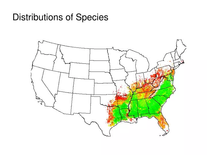
Distributions of Species. How do we represent, methodologically, the distribution of species on the earth? 2. What factors influence the distribution of: Individuals? Populations? Species?. Range Maps – what information do they give us?. There are three basic types: Outline maps

E N D
How do we represent, methodologically, the distribution of species on the earth? • 2. What factors influence the distribution of: • Individuals? • Populations? • Species?
Range Maps – what information do they give us? There are three basic types: Outline maps Dot maps Contour maps
Outline maps show a range as an area, typically shaded, within a boundary. The boundary line defines the limits of the known distribution of the species. Often much guesswork involved. Outline map indicating range of the sooty orange-tip butterfly in Asia.
Dot maps indicate points on a map where a species has been recorded. A dot map showing the locations where the presence of Sonoran Desert canyon ragweed (Ambrosia ambrosioides) has been documented by the collection of a voucher specimen.
Dot and outline maps can be combined. A contour is drawn to enclose the dots, each of which represents a documented location. This is a combination dot and outline map of the distribution of the southern festoon butterfly (Zerynthia polyxena).
Contour maps of the geographic range of the blue jay (Cyanocitta cristata).
Juniper distribution Distribution of Individuals The most basic unit of distribution are individual organisms. It’s generally very difficult to examine that. With some organisms, we can get an idea about the distribution of individuals by looking at aerial photographs.
In Rapoport’s data on palms, the density is much lower at the edge of the distribution and gets progressively greater as one moves into the range. Distributions tend to be complex. Individuals often are found in clumps separated by gaps. As the edge of the range is approached, individuals tend to be more sparsely distributed, with larger gaps.
A depiction of range is scale-dependent. In this depiction of the distribution of Fremont’s leather flower, we can see the range represented on progressively smaller scales, culminating with the distribution of individual plants within a small space. A depiction of range is scale-dependent. In this depiction of the distribution of Fremont’s leather flower, we can see the range represented on progressively smaller scales, culminating with the distribution of individual plants within a small space.
In this example, Population A is intermittently presently and locally extinct. Populations B and C never go locally extinct, but vary dramatically in abundance over time. Abundance and distribution can vary over space and time. This variation can differ among populations.
Distribution of Populations Thomas Malthus, in his 1798 Essay on the Principle of Population, showed that all populations have the capacity to increase in numbers exponentially. The process by which populations change in size can be expressed relatively simply as: r = b + i – d – e where r, the per capita rate of increase, is equal to the sum of the per capita birth rate (b) and the per capita immigration rate (i), minus the per capita mortality rate (d) and the per capita emigration rate (e). Thomas Malthus
When populations are growing exponentially, the rate of growth increases with the population size.
Human population grew at a near exponential rate until recently.
No organisms actually continue to grow at exponential rates. Eventually, they reach a carrying capacity at which the environment is supporting the most individuals possible.
The concept of the ecological niche goes way back, but it was refined by G. Evelyn Hutchinson in 1957 to show how organisms are affected by the physical environment. This diagram depicts a niche in two dimensions. Each dimension reflects an organisms ability to utilize a given range of a physical factor. The resulting two-dimensional figure is a visualization of the organism’s niche with respect to salinity and temperature.
Imagine a fish that utilizes prey size in the frequencies indicated….. … and has O2 requirements as indicated on the Y-axis here. This figure now represents a niche in two dimensions. If we add a third resource, salinity, we can view the niche in three dimensions.
The dashed line on this map of Arizona indicates the northern extent of the distribution of saguaro cactus. The markers represent meteorological stations. The solid points are stations that have never recorded a period of 36 hours without a thaw. The crosses are stations where such periods have been recorded. What does this tell us about the distribution of saguaro cactus? The geographic range of an organism can be viewed as a spatial reflection of its niche.
The term “niche” first appeared in the ecological literature in 1917. At that time, it was used to describe an organism’s physical location in the environment. Charles Elton, in 1927, was the first to use the term in its modern context as the “ecological role” of an organism. This concept is sometimes referred to as an organism’s functional niche. Conditions such as interspecific competition may limit organism’s to only a portion of their fundamental niche. The range of resources actually utilized by an organism is known as its realized niche.
One of the earliest studies examining the ecological niche was done by Joe Connell working with barnacles on the Scottish coast. At Connell’s study site in Scotland, two species of barnacle (Chthalamus stellatus and Balanus balanoides) were commonly found. Although both species settle randomly throughout the intertidal zone, adult Chthalamus are always found higher in the intertidal zone than are Balanus.
Connell performed a series of experiments: • He moved rocks bearing Chthalamus from the upper to the lower intertidal to see whether the species could survive in the low intertidal zone. He also moved rocks bearing Balanus from the low intertidal to the high. • He removed Balanus from rocks in the low intertidal and Chthalamus from rocks in the high intertidal. These experiments were designed to show whether each could grow in the other tidal zone if its competitor were absent.
Niche variables alone are not sufficient to explain patterns of distribution and abundance. • Too simplistic to assume that conditions are equally favorable for a species at all locations where it occurs. Some locations are undoubtedly more favorable than others. In these locations, birth rates will exceed death rates. The surplus individuals can migrate from these “source habitats” to other locales. Other locations may be so unfavorable than death rates exceed birth rates. These sites will be “sink habitats”, and can only continue to exist if they are supplied with immigrants. • There may be sites that are inhabited DESPITE unfavorable environmental conditions. Typically, such situations are explained by the history of the organism at the site. • Other sites may be inhabited intermittently. Local populations are variable, and may occasionally go extinct. The study of such isolated subpopulations has become an area of great interest. The greater population (comprised of the subpopulations) is known as a metapopulation.
While there might be some migration from sink to source habitats, sink habitats must be supported by an influx of individuals from source habitats. This is central to metapopulation theory.
The distribution pattern of most individuals tends to be heterogeneous, with some locations having high densities and others much lower. Such a distribution pattern is called clumped or aggregated.
For both species, only one individual was recorded on the majority of routes. More than 100 were recorded on a limited number of routes. It can be assumed that most of the variation in numbers from one location to another within a distribution results from differences in the degree of suitability of the environmental variables. Common species are usually several orders of magnitude more common at some sites than at others. This can be examined by looking at results of standardized census routes of the North American Breeding Bird Survey.
Rare species may be uncommon throughout their range, but there is still variation. Nancy Rabinowitz identified three “forms” of rarity.
An example can be seen in African locusts. Source populations exist in the darkly shaded areas. These populations are permanent. When conditions are good, they undergo a population “explosion” and spread across South Africa. We may also see temporal variation in distribution and abundance. This typically results from temporal variation in niche parameters.
Winter range of the snowy owl in poor years is indicated by the “dotted” line. Typical range is the darkly shaded area to the north. Similar fluctuations can be seen in other organisms. Voles and lemmings of northern Canada show fluctuations in density ranging across several orders of magnitude. They lack the dispersal ability of locusts. Instead, they show changes in their habitat utilization. Birds that prey on these rodents also show changes in their geographic ranges, shifting far to the south in poor years..
Range Boundaries It appears that the boundary of a species’ range is probably set by multiple environmental factors, some biotic and some abiotic. However, there have been few detailed studies.
As the saguaro cactus approaches the northern edge of its range in the Sonoran desert, it appears to be strongly limited by temperature regime. • Physical factors that play a role in limiting distributions include: • Temperature regime. • Water availability. • Soil and water chemistry.
Many birds seem to be expanding their winter ranges northward as wintertime food becomes more available in the form of bird feeders. However, ecologists have moved away from Leibig’s law of the minimum, and recognized that distributions are influenced by multiple factors. Many birds seem to be limited in the northern extent of their distribution by cold temperatures. This may not be simply the physiological effect of temperature, but its impact on food availability.
Timberline is the upper elevational limit of trees on mountains. Geographically, timberline seems to be related to the mean or maximum temperature during warm months of the growing season. This varies with latitude and elevation. Locally, factors such as wind, snow depth, and energy balance seem to play a role.
Trees at timberline may live for a long time, with very slow growth and infrequent reproduction. Bristlecone pines may live for thousands of years, but grow very slowly. In some places they provide a “fossil timberline”, indicating the elevation that was once suitable for tree growth. Bristlecone pine
The desert pupfish Cyprinodon nevadensis lives in desert streams. Its distribution is strictly limited by temperature. In the outflow stream from a hot spring, it can be found only in areas below 42 C.
Some specialized organisms can be found in places that are not habitable for most animals. Great Salt Lake of Utah supports only two macroscopic inverts, the brine “shrimp” (Artemia salina) and the larvae of the brine fly (Ephydra cinerea). Many other inverts are found in the freshwater streams that empty into the lake, but cannot tolerate the high salinity of the lake itself.
The longleaf pine community is an example of a fire-controlled system. Disturbances of various types also influence local and broadscale distribution patterns. Natural disasters may wipe out entire populations. If they occur regularly, however, they become a natural part of the environment. Situations where there is a regular pattern of colonization and replacement of species following a disturbance illustrate secondary succession (i.e., succession on a location previously inhabited by living things). Fire is an example of a disturbance that has come to be required in many ecological communites.
Periodic disturbance can be severe enough to prevent the expansion of species into areas where they could otherwise survive. Historically, grassland fires have helped prevent the spread of woody vegetation into prairie habitats. In recent years, fire suppression has led to a decrease in the amount of grassland habitat in southern Texas..
Robert Paine found the predation by sea stars on rocky coastlines removed selectively removed the dominant mussels and allowed less effective competitors to coexist with them. Smaller scale disturbances, particularly biological ones like predation, often have the effect of removing dominant species and allowing less dominant species to coexist. This may create a “mosaic” (patchwork) of subhabitats that supports greater diversity.
In many cases, distributions are limited less by physical factors than by biological interactions. The three most significant of these interactions are: 1. Competition. 2. Predation 3. Mutualism African lions and hyaenas may compete for food.
Types of Competition We can classify competitive interactions in a number of ways. The most obvious dichotomy is intraspecific competition, between individuals belonging to the same species, and interspecific competition between individuals of different species. Another extinction can be drawn between exploitation competition, in which the actions of one species (or individual) reduces the availability of a resource to another species and individual, and interference competition, in which the actions of one species (or individual) actively interferes with the abilities of another to use a resource.
Exploitative competition may be consumptive in nature. In America’s southwestern deserts, seed-eating ants compete with rodents like kangaroo rats for a limited number of seeds. This is an example of exploitation competition. Seeds taken by one species are not available for use by the other.
Other examples of preemptive competition may be seen in intertidal invertebrates…… Another form of exploitation competition occurs when organisms compete for space. This is common in plants. If one plant occupies a position in the landscape, it cannot be filled by another plant. This is referred to as preemptive competition.
Exploitation competition may be exemplified by territoriality. In the Cascade Mountains of Washington, two sympatric species of tree squirrels maintain interspecific territories. This ensures both species an adequate food supply. The territory is actively defended. Red squirrel – Tamiasciurus hudsonicus Chickaree – Tamiasciurus douglasii
Interference competition may also take different forms. This include chemical interference, sometimes called allelopathy. Allelopathic organisms release a chemical that has a deletorious effect on other, nearby organisms. Black walnut trees are known for the production of juglone, an allelopathic chemical that interferes with the ability of other plants to establish themselves nearby.
We may also see interference competition in hummingbirds, who may chase other bird away from sources of nectar.
If two species are “complete competitors”, one will win out. This is known as competitive exclusion. It is thought that competitive exclusion may have played a role in the extinction of many prehistoric mammals. For example, the marsupial family Borhyaenidae in South America may have gone extinct after the development of the Panama land bridge enabled North America saber-tooths to enter South America.
Rainbow trout Smoky Mountain stream Competitive exclusion can also be seen in Appalachian streams where the native brook trout can no longer compete with introduced rainbows. Brookies are typically found only in the upper reaches of streams that are unavailable to rainbows. Brook trout
The non-overlapping ranges of five species of large kangaroo rates in the southwestern U.S. probably results from competitive interactions.