Download
1 / 48
480 likes | 539 Views
Explore advanced techniques for rendering implicit surfaces in real-time using GPU acceleration. Dive into root-finding methods, polygonization, and rendering through ray tracing and rasterization. Enhance your understanding of ray-surface intersections and iterative algorithms for implicit function roots. Discover contributions to fluid simulation, fire modeling, and more.

E N D
Jag Mohan Singh IIIT, Hyderabad Real Time Ray-Tracing Implicit Surfaces on the GPU
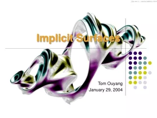
Implicit Surfaces Implicit Surface which can be described by an equation S(x,y,z) = 0. This can be of different kinds Algebraic Non- Algebraic eg. Transcedental, Irrational, Rational etc. • Implicit Surfaces are used for fluid simulation, modeling of fire, waves and natural phenomena described by equations
Thesis Contributions Analytical (Exact) Root Finding at frame-rates of 1100 – 5821 for surfaces up to fourth order Mitchell’s Interval method (first time on GPU) at frame-rates of 60 – 965 for surfaces up to fifth order Marching Points at frame rates of 38 – 825 for arbitrary implicits Adaptive Marching Points (a new method) for arbitrary implicits at frame rates of 60 – 920
Traditional Methods of Rendering Rasterization Ray Tracing
Rendering Implicit Surfaces Polygonization using Marching Cubes Marching Cubes gives a 3d mesh for the input implicit surface Rasterization of this 3d mesh gives the rendering Ray Tracing Shoot rays towards the implicit surface and intersect them with these
Ray-Tracing Implicit Surfaces S(x,y,z) = 0 Ray: P = O + t D t0 Can express as: f(t) = 0 Desired: smallest +ve real root t0 Normal at t0 = (Sx, Sy, Sz) at (O + D t0)
Root Finding Methods Analytical (Exact) exists for polynomials up to fourth order Iterative Methods exists for arbitrary implicits but have problems related to initialization and convergence. Searching based methods which search for the root along the ray using surface properties
Related Work (Exact) Loop and Blinn [ Siggraph ’06] Piecewise algebraic surfaces up to order four. The roots are computed by converting the polynomial to Bezier form. Coefficients are interpolated in vertex shader. If root is inside the Bezier tetrahedron then surface normal and per-pixel lighting done. Problems in quartic root finding due to extreme self intersections Quadric root finding on GPU Sigg , PBG ‘06 Toledo, INRIA Tech Report ‘06 Ranta , ICVGIP ‘06
Iterative Methods Newton Raphson Method xn+1 = xn-f(xn)/ f’ (xn) Laguerre’s method ( Similar to Newton’s) Newton Bisection Method Given interval [t1,t2] Choose one of the intervals [t1,tm] or [tm,t2] where tm is the midpoint
Interval based Iterative Methods Newton’s Interval Method xn+1 = xn- f(xn)/ F’(xn) Krawczyk Method xn+1 = xn-f(xn)/f’(xn) + (I- J( xn) / f’( xn)) (Xn - xn)
Recent Related Work (Iterative) Knoll’s Affine Arithmetic [ CGF ’08] Compute affine extension of function as F If 0 ε F then the interval contains the root Compute maximum depth (dmax) of bisection based on user defined threshold If depth is dmax then we hit the surface Else increment depth and reduce the stepsize by half Back recursion helps in visiting other unvisited nodes in the tree. In the worst case it can lead to visiting all the nodes of the tree.
Related Work (Searching) LG Implicit Surfaces [ Kalra and Barr, Siggraph ’89] Lipschitz constants (L,G) for ray tracing implicits. L is equal to maximum rate of change of f(x) over R. G is equal to maximum rate of change of g(t). Compute Bounding Box (B) divide it into sub-bounding boxes (b) Compute L for b If |f(x0)| > Ld reject b else continue recursive subdivision. For each ray compute bounding box extents t1,t2 and midpoint tm If |g(tm)| > Gd If F(t1) and F(t2) are of opposite signs then find the root using Newton’s method. Else there is no intersection in t1,t2 Else if |g(tm)| < Gd Call the function recursively on intervals [t1,tm] and [tm,t2]
Related Work (Searching) Sphere Tracing [Hart, Visual Computer ’96] Compute while t < D d = f(r(t)) ( Geometric Distance) If d < epsilon then return t t = t + d where Geometric Distance = Signed Distance/ Lipschitz Constant (L)
Roots are computed in power basis Limitations: Not available for polynomials of order > 4! Difficult for non-algebraic equations Must use iterative methods for others Analytical(closed-form) Roots( Our Work)
Analytical Root Finding Cubic Roots Equation (Homogenous Form) : Ax3+3Bx2w+3Cxw2+Dw3 = 0 Compute: δ1= AC-B2 , δ2 = AD-BC, δ3=BD-C2 , δ (discriminant) = 4 δ1 δ3- δ22 The sign of the discriminant and the values of δis determine if it has one triple root, one double and a single real root, three distinct real roots or one real root and one complex conjugate pair as roots.
Analytical Root Finding Quartic Roots The equation is first depressed by removing the cubic term t4+pt2+qt+r = 0 If r is zero then the roots are the roots of cubic equation and zero. If r is non zero then rewrite as (t2+p)2+qt+r = pt2+p2 This is followed by a substitution y s.t. RHS becomes a perfect square (t2+p+y)2 = (p+2y)t2-qt+(y2+2yp+p2-r) Now, for RHS to be a perfect square its discriminant must be zero which yields a cubic equation in y. Now resubstitute to get two quadratic equations.
Interval Arithmetic Two Intervals a = [x, y] and b = [z, w] Addition a + b = [x + z, y + w] Subtraction a – b = [x – w, y – z] Multiplication a * b = [min(xz,xw,yz,yw), max(xz,xw,yz,yw)] Division a/b = a * (1/b) = a* [ 1/w,1/z]
Mitchell’s Interval-Based Method Initialize interval to [ta, tb] = [tnear, tfar] Compute interval extension of function f ([ta, tb]) and it’s derivative ft ([ta, tb]) If f ([ta, tb] contains 0, root exists in it. If ft ([ta, tb]) contains zero, multiple roots. Divide into [ta, tm] and [tm, tb] around the midpoint Recurse into right half only if left has no root. Else, single root. Proceed to root finding Continue till tb -ta < Mitchell, Graphics Interface 90
Interval Extensions Natural: Uses end-points only. f ([ta, tb]) = [min(f(ta), f(tb)), max(f(ta), f(tb))] Centered: f ([ta, tb]) = f (tm) + ft ([ta,tb]) * [ta - tm, tb - tm] Exact: Use critical points ta < t1 < t2 < … < tb of f() f ([ta, tb]) = [min(f(ta), f(t1), f(t2) …, f (tb)), max (f(ta), f(t1), f(t2) …, f(tb))]
Mitchell’s Method: Discussion Advantages: Robust, based on interval arithmetic Fast as the order is logarithmic due to bisections Disadvantages: Good interval extension needed Not obvious for general functions Not easy even for polynomials Difficult on SIMD/GPU Calculations in f(t), derivatives needed Interval extension used is exact
Two-Step Root Finding Bracketing the root Find a (small) bracket/interval that contains the first positive root. Between tnear and tfar Find the root in the interval Newton bisections Always converges, no “special” situations Best for GPU/SIMD as uniform calculations
Marching Points (Sign Test) Divide the parameter domain into equal width intervals from tnear till tfar Compute the function value at endpoints of these intervals. Return the interval with the first sign change.
Marching Points (Taylor Test) • Divide the parameter domain into equal width intervals from tnear till tfar • Compute the values p, q, r and s for an interval and the interval checked for sign change is • [min(p,q,r,s), max(p,q,r,s)]
S(x, y, z) versus f(t) S(x, y, z) is the given form. Relatively simple with dozen or so terms For a given t, evaluate (x, y, z) and S(.). Good for GPU; compose shader on the fly f(t) is different for each ray/pixel. Evaluates to a large number of terms About 1500 terms for a 10th order polynomial Not suitable for GPU/SIMD
Results: Implicit Surfaces (Marching Points)
Marching Points: Discussions Advantages: Easy Implementation Suited for SIMD, fast on current GPUs No need for derivative or coefficient computation Disadvantages: Linear in number of intervals as all may be evaluated Sign Test Not robust. Multiple and close roots are problems No structured way to decide interval size.
Adaptive Marching Points Algebraic distance is used as a measure for searching the root Step-size depends on algebraic distance (S(p(t)) and silhouettes (F’(t))
Adaptive Marching Points Silhouette Adaptation
Self Shadowing Shoot a secondary (shadow) ray towards the light source from intersection point. If this ray intersects the surface in between then the point is in shadow. Only need to bracket the root; no need to find the root.
Dynamic Implicit Surfaces • Implicit Surfaces whose equation varies with time. Blobby Molecules and Twisted Superquadric
Analytic Roots Surface Name FPS for 512x512 Sphere Quadric 5821 Cylinder Quadric 4358 Cayley Cubic 3750 Ding Dong Cubic 3400 Steiner Surface 1400 Tooth Surface 1100 Torus Surface 1200 Surface Name FPS for 512x512 ( Loop and Blinn) Cylinder Quadric 1200 Steiner Surface 500
Mitchell’s Interval Method Surface [Order] Iterations FPS Dervish [5] 86 60 Kiss [5] 65 77 Peninsula [5] 60 85 Cushion [4] 53 170 CrossCap[4] 52 195 Miter [4] 52 186 Tooth[4] 50 195 Cayley [3] 27 580 Ding dong [3] 18 965
Marching Points: Results Surface [Order] Iterations FPS (Sign Test) FPS (Taylor Test) Chmutov [18] 400 85 38 Chmutov[14] 400 55 48 Sarti[12] 300 60 53 Barth [10] 300 92 105 Endreass [8] 300 140 179 Chmutov [8] 250 185 195 Kleine[6] 400 285 290 Hunt [6] 400 230 225 Barth[6] 125 300 310 Heart [6] 120 265 260 Dervish [5] 300 285 275 Peninsula [5] 85 370 447 Torus [4] 50 410 430 Blobby Surface 250 160 305 Scherk’s Surface 250 200 315 Diamond Surface 250 260 306 Superquadric 150 105 125
Adaptive Marching Points: Results Surface [Order] Iterations FPS (Sign Test) FPS (Taylor Test) Chmutov [18] 100 98 60 Chmutov[14] 100 125 95 Sarti[12] 100 86 75 Barth [10] 100 150 115 Endreass [8] 96 190 208 Chmutov [8] 64 215 216 Kleine[6] 48 435 385 Hunt [6] 84 240 325 Barth[6] 60 325 310 Heart[6] 48 420 320 Dervish [5] 45 285 280 Peninsula [5] 35 512 435 Torus [4] 24 555 525 Blobby Surface 50 329 300 Scherk’s Surface 100 358 322 Diamond Surface 100 360 330 Superquadric 100 185 155
Result : Shadows Surface [Order] AMP (Sign Test) AMP (Taylor Test) Without Shadows With Shadows Without Shadows With Shadows Chmutov [18] 98 70 60 45 Chmutov [14] 125 95 95 75 Sarti [12] 86 78 75 49 Barth [10] 150 110 115 79 Endreass[8] 190 140 208 140 Labs[7] 232 165 310 155 Chmutov[6] 418 280 325 235 Hunt[6] 240 182 310 155 Dervish[5] 285 250 280 175 Kiss[5] 428 325 435 265 Tooth[4] 617 425 542 287 Blobby 329 265 300 195 Diamond 360 208 330 199 Superquadric 185 145 155 105
Comparison with Knoll’s Affine Arithmetic Surface FPS (Knoll’s ANE) FPS (AMP Sign) Steiner 38 212 Teardrop 121 178 Tangle 71 196 Barth Sextic 88 120 Kleine 101 170 Mitchell 60 176 Barth Decic 16 94
Results: Robustness Top row: Steiner Surface Bottom row: Cross Cap Surface (Sign Change, Taylor and Interval)
Limitations Chmutov 20 and 30 (Exterior, Interior) • Numerical precision is a issue large number of • roots are present in the exterior of Chmutov • Surface [0.99,1.0] • Taylor test produces false roots for extreme • self intersections (Cushion and Piriform)
What do we need on the GPU? Number format: Exact implementation of IEEE 754 (Limited) Double precision support Beam-Tracing: Transfer roots from one pixel to neighbour Recursive ray-tracing Fixed stack on GPU
Conclusions • MP and AMP methods are widely applicable in terms of Implicit Surfaces and are also SIMD amenable as cost per root finding is low • Analytical Method has limited applicability However it is SIMD amenable • Mitchell’s method has limited applicability and is not SIMD amenable.
Thesis Publications Related Publications GPU Objects Sunil Mohan Ranta , Jag Mohan Singh and P.J. Narayanan Proc. Fifth Indian Conference on Computer Vision, Graphics and Image Processing (ICVGIP), LNCS Volume 4338, Pages 352-363, 2006, Madurai, India Real time Ray tracing of Implicit Surfaces on the GPU Jag Mohan Singh and P. J. Narayanan IEEE Transactions on Visualization and Computer Graphics, 2008 (Under Revision) Other Publications Progressive Decomposition of Point Clouds without Local Planes Jag Mohan Singh and P. J. Narayanan LNCS Volume 4338, Pages 364-375, Proc. of Indian Conference on Computer Vision, Graphics and Image Processing (ICVGIP), 2006 Point Based Representations for Hierarchical EnvironmentsKedarnath Thangudu , Lakshmi Gade,Jag Mohan Singh, and P J Narayanan. Pages 574-578, IEEE Computer Society Press, Proc. of International Conference on Computing: Theory and Applications(ICCTA),2007
CPU and GPU versions Position of Sphere z = 0 z = 1 z = 4 z = 5 GPU Point Sampling 1000 922 790 720 GPU Mitchell 1665.0 1662.0 1662.0 1662.0 CPU Point Sampling 0.8124 0.7939 0.7310 0.7196 CPU Mitchell 2.113 2.113 2.113 2.113 Position of Cubic z = 0 z = 1 z = 4 z = 5 GPU Point Sampling 825.3 724.7 447.5 367.5 GPU Mitchell 955.4 953.4 952.2 952.2 CPU Point Sampling 0.7626 0.7258 0.664 0.656 CPU Mitchell 1.109 1.108 1.108 1.108 Position of Torus z = 0 z = 1 z = 4 z = 5 GPU Point Sampling 410.96 383.77 273.50 230.06 GPU Mitchell 381.06 380.16 379.23 379.23 CPU Point Sampling 0.2202 0.2074 0.1791 0.1759 CPU Mitchell 0.186 0.185 0.185 0.185 Frame Rates for 512x512 Sphere (Quadratic) Ding Dong (Cubic) Torus (Quartic)
Discussion CPU vs GPU SIMD amenable AMP method GPU is able to achieve higher speedups than for Mitchell’s method. Interval method is faster for lower order surfaces than AMP. This advantage is nullified for higher order surfaces.