Download
1 / 22
230 likes | 440 Views
ANOVA Single Factor Models. ANOVA. ANOVA ( AN alysis O f VA riance) is a natural extension used to compare the means more than 2 populations.

E N D
ANOVA Single Factor Models
ANOVA • ANOVA (ANalysis Of VAriance) is a natural extension used to compare the means more than 2 populations. • Basic Question: Even if the true means of n populations were equal (i.e. m1 = m2 = m3 = m4) we cannot expect the sample means (x1, x2, x3, x4 ) to be equal. So when we get different values for the x’s, • How much is due to randomness? • How much is due to the fact that we are sampling from different populations with possibly different mj’s.
ANOVA TERMINOLOGY • Response Variable (y) • What we are measuring • Experimental Units • The individual unit that we will measure • Factors • Independent variables whose values can change to affect the outcome of the response variable, y • Levels of Factors • Values of the factors • Treatments • The combination of the levels of the factors applied to an experimental unit
Example We want to know how combinations of different amounts of water (1 ac-ft, 3 ac-ft, 5 ac-ft) and different fertilizers (A, B, C) affect crop yields • Response variable – crop yield (bushels/acre) • Experimental unit • Each acre that receives a treatment • Factors (2) • Water and fertilizer • Levels (3 for Water; 3 for Fertilizer) • Water: 1, 3, 5; Fertilizer: A, B, C • Treatments (9 = 3x3) • 1A, 3A, 5A, 1B, 3B, 5B, 1C, 3C, 5C
Single Factor ANOVABasic Assumptions • If we focus on only one factor (e.g. fertilizer type in the previous example), this is called single factor ANOVA. • In this case, levels and treatments are the same thing since there are no combinations between factors. • Assumptions for Single Factor ANOVA • The distribution of each population in the comparison has a normal distribution • The standard deviations of each population (although unknown) are assumed to be equal (i.e. s1 = s2 = s3 = s4) • Sampling is: Random Independent
Example • The university would like to know if the delivery mode of the introductory statistics class affects the performance in the class as measured by the scores on the final exam. • The class is given in four different formats: • Lecture • Text Reading • Videotape • Internet • The final exam scores from random samples of students from each of the four teaching formats was recorded.
Summary • There is a single factor under observation – teaching format • There are k = 4 different treatments (or levels of teaching formats) • The number of observations (experimental units) are n1 = 7, n2 = 8, n3 = 6, n4 = 5 total number of observations, n = 26
Why aren’t all thex’s the same? • There is variability due to the different treatments -- Between Treatment Variability(Treatment) • There is variability due to randomness within each treatment -- Within Treatment Variability(Error) BASIC CONCEPT If the average Between Treatment Variability is “large” compared to the average Within Treatment Variability, we can reasonably conclude that there really are differences among the population means (i.e. at least one μj differs from the others).
Basic Questions • Given this basic concept, the natural questions are: • What is “variability” due to treatment and due to error and how are they measured? • What is “average variability” due to treatment and due to error and how are they measured? • What is “large”? • How much larger than the observed average variability due to error does the observed average variability due to treatment have to be before we are convinced that there are differences in the true population means (the µ’s)?
How Is “Total” Variability Measured? Variability is defined as the Sum of Square Deviations (from the grand mean). So, SST(Total Sum of Squares) • Sum of Squared Deviations of all observations from the grand mean. (McClave uses SSTotal) • SSTr(Between Treatment Sum of Squares) • Sum of Square Deviations Due to Different Treatments. (McClave uses SST) • SSE(Within Treatment Sum of Squares) • Sum of Square Deviations Due to Error SST = SSTr + SSE
How is “Average” Variability Measured? • VariabilitySSDFMean Square (MS) • Between Tr. (Treatment) SSTr k-1 SSTr/DFTR • Within Tr. (Error) SSE n-k SSE/DFE • TOTAL SST n-1 ANOVA TABLE # treatments -1 DFT - DFTR # observations -1 “Average” Variability is measured in: Mean Square Values (MSTr and MSE) • Found by dividing SSTr and SSE by their respective degrees of freedom
Formula for CalculatingSST Calculating SST Just like the numerator of the variance assuming all (26) entries come from one population
Formula for Calculating SSTr Calculating SSTr Between Treatment Variability Replace all entries within each treatment by its mean – now all the variability is between (not within) treatments 76 76 76 76 76 76 76 65 65 65 65 65 65 65 65 75 75 75 75 75 75 74 74 74 74 74
Formula for Calculating SSE Calculating SSE (Within Treatment Variability) The difference between the SST and SSTr ---
Can we Conclude a Difference Among the 4 Teaching Formats? We conclude that at least one population mean differs from the others if the average between treatment variability is large compared to the average within treatment variability, that is if MSTr/MSE is “large”. • The ratio of the two measures of variability for these normally distributed random variables has an F distribution and the F-statistic (=MSTr/MSE) is compared to a critical F-value from an F distribution with: • Numerator degrees of freedom = DFTr • Denominator degrees of freedom = DFE • If the ratio of MSTr to MSE (the F-statistic) exceeds the critical F-value, we can conclude that at least one population mean differs from the others.
Can We Conclude Different Teaching Formats Affect Final Exam Scores?The F-test H0: m1 = m2 = m3 = m4 HA: At least one mj differs from the others Select α = .05. Reject H0 (Accept HA) if:
Hand Calculations for the F-test Cannot conclude there is a difference among the μj’s
EXCEL OUTPUT p-value = .365975 > .05 Cannot conclude differences
REVIEW • ANOVA Situation and Terminology • Response variable, Experimental Units, Factors, Levels, Treatments, Error • Basic Concept • If the “average variability” between treatments is “a lot” greater than the “average variability” due to error – conclude that at least one mean differs from the others. • Single Factor Analysis • By Hand • By Excel