Download
1 / 58
610 likes | 1.35k Views
Chapter 12 Linear Regression and Correlation. General Objectives:

E N D
Chapter 12 Linear Regression and Correlation General Objectives: In this chapter we consider the situation in which the mean value of a random variable y is related to another variable x. By measuring both y and x for each experimental unit, thereby generating bivariate data, you can use the information provided by x to estimate the average value of y for preassigned values of x. ©1998 Brooks/Cole Publishing/ITP
Specific Topics 1. A simple linear probabilistic model 2. The method of least squares 3. Analysis of variance for linear regression 4. Testing the usefulness of the linear regression model: inferences about b, The ANOVA F Test, and r2 5. Estimation and prediction using the fitted line 6. Diagnostic tools for checking the regression assumptions 7. Correlation analysis ©1998 Brooks/Cole Publishing/ITP
12.1 Introduction • You would expect the college achievement of a student to be a function of several variables: - Rank in high school class - High school’s overall rating - High school GPA - SAT scores • The objective is to create a prediction equation that expresses y as a function of these independent variables. • This problem was addressed in the discussion of bivariate data. • We used the equation a straight line to describe the relationship between x and y and we described the strength of the relation-ship using the correlation coefficient r. ©1998 Brooks/Cole Publishing/ITP
12.2 A Simple Linear Probabilistic Model • In predicting the value of a response y based on the value of an independent variable x, the best-fitting line y =a +bx is based on a sample of n bivariate observations drawn from a larger population of measurements, e.g., the height and weight of 100 male students at a given university. • To construct a population model to describe the relationship between y and x, assume that y is linearly related to x. • Use the deterministic model y = a+ bx where a is the y-intercept, the value of y when x =0 and b is the slope of the line, as shown in Figure 12.1. ©1998 Brooks/Cole Publishing/ITP
Table 12.1 displays the math achievement test scores for a random sample of n = 10 college freshmen, along with their final calculus grades. A plot appears in Figure 12.2. Table 12.1 Mathematics Final Achievement Calculus Student Test Score Grade 1 39 65 2 43 78 3 21 52 4 64 82 5 57 92 6 47 89 7 28 73 8 75 98 9 34 56 10 52 75 ©1998 Brooks/Cole Publishing/ITP
Figure 12.2Scatterplot of the data in Table 12.1 ©1998 Brooks/Cole Publishing/ITP
Notice that the points do not lie exactly on a line, but rather seem to be deviations about an underlying line. • A simple way to modify the deterministic model is to add a random error component to explain the deviations of the points about the line. • A particular response y is described using the probabilistic model y = a+ bx+ e . • The first part of the equation, a+ bx—called the line of means— describes the average of y for a given value of x. • The error component e allows each individual response y to deviate from the line of means by a small amount. ©1998 Brooks/Cole Publishing/ITP
Assumptions About the Random Error: Assume that the values of e satisfy these conditions: - Are independent in the probabilistic sense - Have a mean of 0 and a common variance equal to s 2 - Have a normal probability distribution • These assumptions about the random error e are shown in Figure 12.3 for three fixed values of x. • You can use sample information to estimate the values of aand b, which are the coefficients of the line of means, • These estimates are used to form the best-fitting line for a given set of data, called the least squares line or regression line. ©1998 Brooks/Cole Publishing/ITP
Figure 12.3Linear probabilistic model ©1998 Brooks/Cole Publishing/ITP
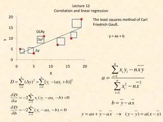
12.3 The Method of Least Squares • The formula for the best-fitting line is where a and b are the estimates of the intercept and slope parameters aand b, respectively. • The fitted line for the data in Table 12.1 is shown in Figure 12.4. • The vertical lines drawn from the prediction line to each point represent the deviations of the points from the line. ©1998 Brooks/Cole Publishing/ITP
Figure 12.4Graph of the fitted line and data points in Table 12.1 ©1998 Brooks/Cole Publishing/ITP
Principle of Least Squares: The line that minimizes the sum of squares of the deviations of the observed values of y from those predicted is the best-fitting line. The sum of squared deviations is commonly called the sum of squares for error (SSE) and defined as • In Figure 12.4, SSE is the sum of the squared distances represented by the vertical lines. • a and b are called the least squared estimators of aand b . ©1998 Brooks/Cole Publishing/ITP
Least Squares Estimators of a and b : where the quantities Sxy and Sxx are defined as and • The sum of squares of the x values is found using the shortcut formula in Chapter 2. • The sum of the cross-products is the numerator of the covariance defined in Chapter 3. (See Example 12.1 on page 519.) ©1998 Brooks/Cole Publishing/ITP
Making sure that calculations are correct: - Be careful of rounding errors. - Use a scientific or graphing calculator - Use computer software. - Always plot the data and graph the line.
12.4 An Analysis of Variance for Linear Regression • In a regression analysis, the response y is related to the independent variable x. • The total variation in the response variable y, given by is divided into two portions: - SSR (sum of squares regression) measures the amount of variation explained by using the regression line with one independent variable x - SSE (sum of squares error) measures the “residual” variation in the data that is not explained by the independent variable x ©1998 Brooks/Cole Publishing/ITP
You have: Total SS = SSR + SSE • For a particular value of the response yi, you can visualize this breakdown in the variation using the vertical distances illustrated in Figure 12.5: ©1998 Brooks/Cole Publishing/ITP
SSR is the sum of the squared deviations of the differences between the estimated response without using x and the estimated response using x • It is not too hard to show algebraically that • Since Total SS = SSR + SSE, you can complete the partition by calculating ©1998 Brooks/Cole Publishing/ITP
Each of the sources of variation, divided by the degrees of freedom, provides an estimate of the variation in the experiment. • These estimates are called mean squares, MS=SS/df and are displayed in an ANOVA table as shown in Table 12.3 for the general case. • The total number of df is n - 1. • There is one degree of freedom associated with SSR since the regression line involves estimating one additional parameter. • SSE has n - 2df. • The mean square error MSE= s2=SSE/(n - 2) is an unbiased estimator of the underlying variance s2. ©1998 Brooks/Cole Publishing/ITP
The first two lines in Figure 12.6 give the least squares line. • The best unbiased estimate of • The best unbiased estimate of s is • This measures the unexplained or “leftover” variation in the experiment. ©1998 Brooks/Cole Publishing/ITP
12.5 Testing the Usefulness of the Linear Regression Model • In considering linear regression, you may ask two questions: - Is the independent variable x useful in predicting the response variable y? - If so, how well does it work? • Inferences concerning b. The Slope of the Line of Means - It can be shown that, if the assumptions about the random error e are valid, then the estimator b has a normal distribution in repeated sampling with E(b) =b and standard error given by where s2 is the variance of the random error e. ©1998 Brooks/Cole Publishing/ITP
Since the value of s2 is estimated with s2= MSE, you can base inferences on the statistic given by which has a t distribution with df = (n - 2), the degrees of freedom associated with MSE. Test the Hypothesis Concerning the Slope of a Line: 1. Null hypothesis: H0 : b=b0 2. Alternative hypothesis: One-Tailed Test Two-Tailed Test Ha : b>b0Ha : b¹b0 (or Ha : b<b0) 3. Test statistic: ©1998 Brooks/Cole Publishing/ITP
When the assumptions given in Section 12.2 are satisfied, the test statistic will have a Student’s t distribution with (n - 2) degrees of freedom. 4. Rejection region: Reject H0 when One-Tailed Test Two-Tailed Test t>tat >ta/2 or t<-ta/2 (or t<-ta when the alternative hypothesis is Ha : b<b0) or when p value < a ©1998 Brooks/Cole Publishing/ITP
See Example 12.2 for an example of a test for a linear relationship. Example 12.2 Determine whether there is a significant linear relationship between the calculus grades and test scores listed in Table 12.1. Test at the 5% level of significance. Solution The hypotheses to be tested are H0 : b= 0 versus H0 : b¹ 0 and the observed value of the test statistic is calculated as with (n - 2) = 8 degrees of freedom. ©1998 Brooks/Cole Publishing/ITP
With a=.05, you can reject H0 when t> 2.306 or t< -2.306. Since the observed value of the test statistic falls into the rejection region, H0 is rejected and you can conclude that there is a significant linear relationship between the calculus grades and the test scores for the population of college freshmen. ©1998 Brooks/Cole Publishing/ITP
Table 12.1 Mathematics Final Achievement Calculus Student Test Score Grade 1 39 65 2 43 78 3 21 52 4 64 82 5 57 92 6 47 89 7 28 73 8 75 98 9 34 56 10 52 75 ©1998 Brooks/Cole Publishing/ITP
A (1 -a)100% Confidence Interval for b : b±ta/2(SE) where ta/2 is based on (n - 2) degrees of freedom and • See Example 12.3 for the calculation of confidence intervals. Example 12.3 Find a 95% confidenceinterval estimate of the slope b for the calculus grade data in Table 12.1. Solution Substituting previously calculated values into ©1998 Brooks/Cole Publishing/ITP
The resulting 95% confidence interval is .362 to 1.170. Since the interval does not contain 0, you can conclude that the true value of b is not 0, and you can reject the null hypothesis H0 : b= 0 in favor of Ha : b¹ 0, a conclusion that agrees with the findings in Example 12.2. Furthermore, the confidence interval estimate indicates that there is an increase of from as little as .4 to as much as 1.2 points in a calculus test score for each 1-point increase in the achievement test scores. ©1998 Brooks/Cole Publishing/ITP
A Minitab regression analysis appears in Figure 12.7. This matches Example 12.2. Figure 12.7 ©1998 Brooks/Cole Publishing/ITP
The Analysis of Variance FTest In Figure 12.7, F = MSR/MSE = 19.14 with 1 df for the numerator and (n - 2) = 8 df for the denominator. ©1998 Brooks/Cole Publishing/ITP
Measuring the Strength of the Relationship:The Coefficient of Determination • To determine how well the regression model fits, you can use a measure related to the correlation coefficient r: • The coefficient of determination is the proportion of the total variation that is explained by the linear regression of y on x. • Since Total SS =Syy and SSR =Syx/Sxx, you can write ©1998 Brooks/Cole Publishing/ITP
Definition: The coefficient of determinationr2 can be interpreted as the percent reduction in the total variation in the experiment obtained by using the regression line =a + bx, instead of ignoring x and using the sample mean to predict the response variable y. Interpreting the Results of a Significant Regression • Even if you do reject the null hypothesis that the slope of the line equals 0, it does not necessarily mean that y and x are unrelated. • It may be that you have committed a Type II error—falsely declaring that the slope is 0 and that x and y are unrelated. ©1998 Brooks/Cole Publishing/ITP
Fitting the Wrong Model - It may happen that y and x are perfectly related in a nonlinear way as in Figure 12.8. Figure 12.8 ©1998 Brooks/Cole Publishing/ITP
Here are the possibilities: - If observations were taken only with the interval b < x < c, the relationship would appear to be linear with a positive slope. - If observations were taken only with the interval d < x < f, the relationship would appear to be linear with a negative slope. - If observations were taken over the interval c < x < d, the line would be fitted with a slope close to 0, indicating no linear relationship between y and x. ©1998 Brooks/Cole Publishing/ITP
Extrapolation - Problem: To apply the results of a linear regression analysis to values of x that are not included within the range of the fitted data. - Extrapolation can lead to serious errors in prediction, as shown in Figure 12.8. • Causality - A significant regression implies that a relationship exists and that it may be possible to predict one variable with another. - However, this in no way implies that one variable causes the other variable. ©1998 Brooks/Cole Publishing/ITP
12.6 Estimation and Prediction Using the Fitted Line • Now that you have tested the fitted regression lineto make sure that it is useful for prediction, you can use it for one of two purposes: - Estimating the average value of y for a given value of x - Predicting a particular value of y for a given value of x • The average value of y is related to x by the line of means shown as a broken line in Figure 12.9. ©1998 Brooks/Cole Publishing/ITP
Figure 12.9 Distribution of y for x = x0 ©1998 Brooks/Cole Publishing/ITP
Since the computed values of a and b vary from sample to sample, each new sample produces a different regression line, which can be used either to estimate the line of means or to predict a particular value of y. • Figure 12.10 shows one of the possible configurations of the fitted line, the unknown line of means, and a particular value of y. • The variability of our estimator is measured by its standard error. • is normally distributed with standard error of estimated by ©1998 Brooks/Cole Publishing/ITP
Figure 12.10 Error in estimating E(y|x) and in predicting y ©1998 Brooks/Cole Publishing/ITP
Estimation and testing are based on the statistic • You can use the usual form for a confidence interval based on the t distribution: • If you examine Figure 12.10, you can see that the error in prediction has two components: - The error in using the fitted line to estimate the line of means - The error caused by the deviation of y from the line of means, measured by s2 • The variance of the difference between y and is the sum of these two variances and forms the basis for the standard error (y - ) used for prediction: ©1998 Brooks/Cole Publishing/ITP
(1 - a)100% Confidence and Prediction Intervals • For estimating the average value of y when x = x0 : • For predicting a particular value of y when x = x0 : where ta/2 is the value of t with (n- 2)degrees of freedom and area a/2 to its right. ©1998 Brooks/Cole Publishing/ITP
The test for a 0 intercept is given in Figure 12.11: • The Minitab regression command provides an option for either estimation or prediction. See Figure 12.12: ©1998 Brooks/Cole Publishing/ITP
The confidence bands and prediction bands generated by Minitab for the calculus grades data are shown in Figure 12.13: ©1998 Brooks/Cole Publishing/ITP
12.7 Revisiting the Regression Assumptions Regression Assumptions: - The relationship between y and x must be linear, given by the model - The values of the random error term e (1) are independent, (2) have a mean of 0 and a common variance s 2, indepen- dent of x, and (3)are normally distributed. • The diagnostic tools for checking these assumptions are the same as those used in Chapter 11, based on the analysis of the residual error. • When the error terms are collected at regular time intervals, they may be dependent, and the observations make up a time series whose error terms are correlated. ©1998 Brooks/Cole Publishing/ITP
Other regression assumptions can be checked using residual plots. • You can use the plot of residuals versus fit to check for a constant variance as well as to make sure that the linear model is in fact adequate. See Figure 12.14: ©1998 Brooks/Cole Publishing/ITP
The normal probability plot is a graph that plots the residuals against the expected value of that residual if it had come from a normal distribution. • The normal probability plot for the residuals in Example 12.1 is given in Figure 12.15: ©1998 Brooks/Cole Publishing/ITP
12.8 Correlation Analysis Pearson Product Moment Coefficient of Correlation: • The variances and covariances are given by: • In general, when a sample of n individuals or experimental units is selected and two variables are measured on each individual or unit so that both variables are random, the correlation coef-ficient r is the appropriate measure of linearity for use in this situation. See Examples 12.7 and Table 12.4. ©1998 Brooks/Cole Publishing/ITP
Example 12.7 The heights and weights of n= 10 offensive backfield football players are randomly selected from a county’s football all-stars. Calculate the correlation coefficient for the heights (in inches) and weights (in pounds) given in Table 12.4. Solution You should use the appropriate data entry method of your scientific calculator to verify the calculations for the sums of squares and cross-products: using the calculational formulas given earlier in this chapter. Then or r =.83. This value of r is fairly close to 1, the largest possible value of r , which indicates a fairly strong positive linear relationship between height and weight. ©1998 Brooks/Cole Publishing/ITP
Table 12.4 Heights and weights of n= 10 backfield all-stars Player Height x Weight y 1 73 185 2 71 175 3 75 200 4 72 210 5 72 190 6 75 195 7 67 150 8 69 170 9 71 180 10 69 175 ©1998 Brooks/Cole Publishing/ITP
There is a direct relationship between the calculation formulas for the correlation coefficient r and the slope of the regression line b. • Since the numerator of both quantities is Sxy, both r and b have the same sign. • Therefore, the correlation coefficient has these general properties: - When r =0, the slope is 0, and there is no linear relationship between x and y. - When r is positive, so is b, and there is a positive relationship between x and y. - When r is negative, so is b, and there is a negative relationship between x and y. • Figure 12.16 shows four typical scatter plots and their associated correlation coefficients. ©1998 Brooks/Cole Publishing/ITP
Figure 12.16 Some typical scatterplots ©1998 Brooks/Cole Publishing/ITP