Download
1 / 35
350 likes | 894 Views
Steve Cunningham. 3D Computer Graphics and Universal Supercomputers.

E N D
Steve Cunningham 3D Computer Graphics and Universal Supercomputers
3D computer graphics is an enormous consumer of computing resources, and the market has responded to the continuing growth in demand for high-performance graphics by creating continually more powerful graphics processors. We will trace these parallel paths from the point where 3D graphics began to replace 2D graphics to the near-future state of 3D graphics, and show how the graphics processor is leading us to having usable laptop and desktop supercomputers.
1970s – graphics standards were 2D (GSPC, GKS), with 3D graphics in labs and research. Many fundamental algorithms and techniques were developed and the graphics pipeline became well understood. A few weak 3D standards were developed. 1980s – Silicon Graphics was founded in 1981. It was unique because of its geometry engine, a VLSI implementation of the graphics pipeline. SGI created the Iris GL graphics API to access the power of the Iris workstations. 1990s -- SGI opened up GL to create the OpenGL system in 1992. OpenGL was originally often software-only, perhaps with a floating-point accelerator. The first graphics cards were released that incorporated more and more of the graphics pipeline in silicon. Other APIs also created, usually similar to OpenGL. However, OpenGL could not do some of the 1970s techniques. A Quick Review of 40 Years of Graphics
2000s – OpenGL implementations were found to be less powerful than desired, especially for games, and the system was expanded by developing programmable shaders that could move more and more functionality to special silicon and allow the programmer to create new techniques. 2010s – the “fixed-function” pipeline of the 1980s-2000s began to go away (e.g. OpenGL ES, OpenGL 3.0) and developers began to need to create all their graphics functionality in programmable shaders. The resulting graphics cards became less and less graphics cards and more and more parallel coprocessor cards, and APIs for general parallel programming on them became available (CUDA, OpenCL, others) A Quick Review of 40 Years of Graphics
Let’s look at the graphics pipeline and, once we understand how that works, see how we can speed up pipeline processing by using silicon. So...
The graphics pipeline has two parts • The geometry pipeline • You define the original geometry of your scene, and this is transformed into the 2D geometry of the scene with vertex properties. • The rendering pipeline • Starting with the geometry of the 2D scene, the full set of pixels for the scene is created. The Graphics Pipeline
The Geometry Pipeline This is the space in which you define your graphics objects based on a simple set of polygon-based graphics primitives. The coordinates are independent of the final world your graphics will appear in, so you can think of these objects as templates rather than final entities. Model Space
The Geometry Pipeline Modeling Transformation World space is the common space in which all your scene is organized, and modeling transformations take the original models and place them in this space. Modeling transformations include scaling, rotation, and translation, and all involve 4x4 matrix multiplications. Actual systems create a single modeling transformation for each graphics primitive. Model Space World Space
The Geometry Pipeline Modeling Transformation Viewing Transformation Model Space World Space Eye Space Eye space is the world space with the origin moved to the eyepoint and the z-axis aligned with the direction of the view. The viewing transformation is calculated as a 4x4 matrix (for compatibility with modeling transformations) and the modeling and viewing matrices are multiplied to give a modelview matrix for each primitive.
The Geometry Pipeline Modeling Transformation Viewing Transformation Projection Transformation Model Space World Space Eye Space 2D Space Screen space is the eye space projected down into a 2D space in a standard way (e.g. perspective). The projection transformation is also managed as a matrix, and the projection and modelview matrices are multiplied to give a modelviewprojection matrix for each primitive. Vertices in screen space usually have other properties besides their (x,y) coordinates. These include depth (retained from eye space) and attributes such as color or texture coordinates. Many of these properties are computed from program parameters (lights, materials, ...)
Some key features of this pipeline process: • Involves a large number of matrix operations • Each vertex of each primitive is fully multiplied. • Involves potentially changing the matrices for each graphics primitive: • The modeling transformation may change, changing the modelviewprojection matrix. • The change is managed efficiently. • Involves possibly complex lighting computations. • Except for changing the matrices, this process is exactly the same for each vertex (hint, hint...) The Geometry Pipeline
We start with graphics primitives in 2D space as produced by the geometry pipeline. Each primitive is definec by its vertices with (x,y) coordinates, depth, and likely other attributes (e.g. color, texture coordinates, ...). Each primitive is to be rendered as a collection of colored pixels. The key process for rendering is interpolation of the vertex properties. The Rendering Pipeline
The first step is to convert the primitive’s 2D vertices to screen (integer) coordinates. Between each adjacent pair of vertices, compute the pixels for that edge. The Rendering Pipeline • Edge computation can use several different interpolation algorithms and many vertex attributes are interpolated.
Once we have created the edges, we interpolate across the interior of the primitive. The Rendering Pipeline • The vertex attributes are simultaneously interpolated across the interior.
As we render a primitive, we can integrate it with the other things we already have in an image buffer: • visibility testing • color blending • This process is called primitive assembly The Rendering Pipeline
The things we typically interpolate are • depth (used for depth testing) • color (smooth shading) • including interpolating the alpha value if needed • texture coordinates • fog parameters • Everything is a simple linear interpolation. The Rendering Pipeline
These interpolation processes can be slow: • pixel addresses are integer, but the data being interpolated is usually real. • some of the processes (e.g. texture mapping) involve doing a lookup of one or more values in an array. • But, similarly to the geometry pipeline, the processes are the same for each pixel. The Rendering Pipeline
Enter, update, and multiply 4x4 matrices, Multiply 4D vectors by 4x4 matrices, Compute lighting values for each pixel, Interpolate real values across integer spaces, Look up values in good-sized arrays, Compute pixel color from texture operations, Merge computed values with existing values in storage. Let’s Summarize the Pipeline Operations
Minimal support: floating-point hardware (students, ask the faculty; this is ancient history!) and all the operations are done by the CPU in main memory. How Are These Operations Supported?
Better support: use a graphics processor (card) that supports the pipeline. • Geometry pipeline: • Pass the transformations into the card, • Pass the vertices into the card, • Multiply vertices by transformation, • Compute lighting for each vertex, • Assemble the set of 2D vertices. • Problems: complex lighting operations and communications bandwidth to the card. How Are These Operations Supported?
Rendering pipeline: • Take the primitive that was assembled (2D vertices in sequence, with lighting and other data). • Interpolate the data (2D position, color, texture coordinates, depth, fog parameters, ...) and do the texture lookups and computations to compute the data for each pixel. • Carry out the pixel processing (depth testing, blending, texture lookup, ...) for the output buffer. • Problem: the pixel processing can be quite complex (e.g. multiple textures, complex texture operations, ...) How Are These Operations Supported?
Certainly speeded up the graphics pipeline. Had to be complex to handle the many options for lighting and texture operations. Had some limitations for handling interpolations. Had some limitations for handling pixel. operations They supported OpenGL well at the 1.2 level or so. So Early Graphics Cards
Worked on two particular parts of the problem: • Minimized data transfer to the card. • Let you send vertex arrays to the card rather than single vertices. • Supported “compiled graphics” where the results of operations were retained by the card. • Handled pixel operations more fluently. • Improved the size and communications with texture memory. • Improved other details of pixel operations. • Developments paralleled fixed-function OpenGL. The Next Generation of Graphics Cards
Shaders are programs written to run on a graphics card and replace some part of the fixed-function pipeline. • At this point there are three kinds of shaders: • Vertex shaders: replace part of the geometry pipeline. • Fragment shaders: replace part of the rendering pipeline. • Geometry shaders: create new geometry in the geometry pipeline. Then Came Graphics Shaders
Operate STRICTLY one vertex at a time. Take the original position of the vertex and other properties (normal, color, lights, ...) Output the position and color of the vertex after processing, any other changed properties. Vertex Shaders
Take a “primitive with adjacency” (so, more than one vertex) plus other properties. Allow you to create new geometry from the original adjacency information. Geometry Shaders
Interpolate the vertices in a 2D primitive to fill each pixel contained in the primitive. Texturing and many other kinds of computation can be done. Fragment Shaders
Designed to match OpenGL 2.1 Many individual processors on the card (>128). Specialized access pathways for data in texture arrays. Continuing to support the fixed-function pipeline requires a lot of fixed operations on the card. Cards that Support Shader Programming
Continuing to support the fixed-function pipeline puts an overhead on the graphics card that reduces its capabilities. Some devices simply do not have enough capability to handle the fixed-function operations. This is great ... but
In the embedded-systems version of OpenGL, OpenGL ES, shaders are not an option – they are required. The fixed-function pipeline is simply not there. In OpenGL 3, the fixed-function pipeline is deprecated in favor of all-shader graphics. The graphics processors for this new level of graphics are intended to be self-contained. Because of this ...
Will not have special fixed-function capabilities Will take large-scale data input (as used for vertex arrays and large textures). Will operate on (narrow) parallel arrays (as used for vertex, vector, and array operations). Will support arbitrary computations. Will operate at very high speeds. The general concept is called GPGPU: general programming on a GPU. So the New Graphics Cards
... are really vector supercomputers, with very large on-board data storage and very fast parallel operations. But how do you use these capabilities for anything besides graphics? These Graphics Cards ...
There is a new family of APIs that give programmers access to the cards’ power • CUDA (nVIDIA specific) • various language bindings, including pyCUDA • OpenCL looks to be more designed to run on a wider variety of hardware To Support This Computation
Not because this is a stopping place, but because it is a starting place for a new paradigm and a new set of tools. I cannot take you into this new land, but I can see into it and offer you a very interesting future. I believe you will find this a very exciting place to work. We Stop Here...