Distributions in space

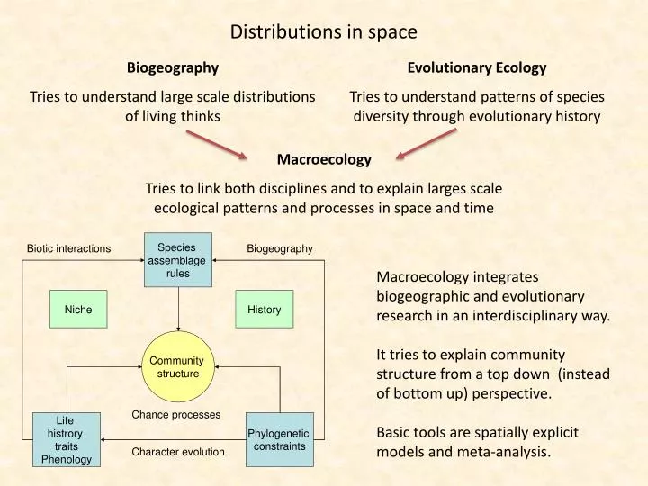
1. Distributions in space Biogeography Tries to understand large scale distributions of living thinks Evolutionary Ecology Tries to understand patterns of species diversity through evolutionary history Macroecology Tries to link both disciplines and to explain larges scale ecological patterns and processes in space and time Macroecology integrates biogeographic and evolutionary research in an interdisciplinary way. It tries to explain community structure from a top down (instead of bottom up) perspective. Basic tools are spatially explicit models and meta-analysis.

2. Ecological processes Evolutionaryprocesses Speciation ExtinctionClimatic processes Dispersal MetapopulationsMetacommunities Evolutionary processes Ecological processes FluctuationsLocal species turnover Speciation ExtinctionGeological processes PredationDisturbanceCompetition Dispersal MetapopulationsSpatial processes

3. Theory of Island biogeography The Galapagos Islands Robert MacArthur (1930-1972) Edward O. Wilson(1929-) One islands Two islands Immigration Extinction Immigration Extinction near small Equilibrium species richness Equilibrium species richness far large Rate Rate Species richness Species richness The theory of island biogeography tries to understand species diversity on all sorts of isolated islands from stochastic colonization of islands and random extinction on islands. Colonization rates depend on island area and isolation. Extinction rates depend on island area only. The model is species based

4. Theory of Island biogeography S = S0e-kI Species richness Species richness S = S0Az Isolation Area The species – isolation relationship The species – area relationship Avifauna of New Guinea Land plant of Britain from Watson (1859) Diamond 1972, PNAS 69: 3199-3203

5. The increase of speciesrichness with samplesize Speciesrichness on deepseamounts, Forges 2000 ParasitoidHymenoptera on a drymeadow on limestone, Ulrich 2005 Butterflycatches by Preston 1948 Increase of land plant families in evolutionarytime, Knoll 1986 Increase of herbivoreson bracken, Lawton 1986

6. The power function species – sample size relationship The species – area - time relationship The species – area relationship The species – time relationship • The number of species counts increases with area and time. • This relationship often follows a power function • The slope z of this function measures how fast species richness increases with increasing area. It is therefore a measure of spatial species turnrover or beta diversity • The intercept S0 is a measure of the expected number of species per unit of area. It is therefore a measure of alpha diversity • Changes in slope through time point to disturbances like habitat fragmentation or destruction • The slope of the species – time relationship is a measure of local species extinction rate. Collembolan species richness across Europe

7. 700 600 1.4 A B C 600 1.3 500 1.2 500 400 1.1 400 Turnover Number of species Number of species 300 300 1 200 200 0.9 100 0.8 100 0.7 0 0 0 5 10 0 50 100 150 0 50 100 150 Area Area t The species – time relationship Local species area and species time relationships in a temperate Hymenoptera community studied over a period of eight years. S = S0Az S = S0tt S = S0Aztt The accumulation of species richness in space and time follws a power function model Coeloidespissodis (Braconidae) The mean extinction rate per year is about 9% S = (73.0±1.7)A(0.41±0.01) t(0.094±0.01)

8. 10000 between biotas: z = 0.53 1000 Number of species 100 within a regional pool: z = 0.09 10 small areas: z = 0.43 1 1.0E-01 1.0E+01 1.0E+03 1.0E+05 1.0E+07 1.0E+09 1.0E+11 1.0E+13 Area [Acres] Species - area relationship of the world birds at different scales Preston 1960, Ecology 41: 611-67 RegionalSARshaveslopesbetween 0.1 and 0.3. Local and continentalSARshaveslopes > 0.25.

9. 1000000 Intercontinental scale: z = 0.5 100000 10000 Number of species 1000 100 Regional scale: z = 0.14 10 Local scale: z = 0.25 1 1.E-04 1.E-02 1.E+00 1.E+02 1.E+04 1.E+06 1.E+08 1.E+10 1.E+12 2 Area [km ] The species – area relationship of plants follows a three step pattern as in birds Shmida, Wilson 1985, J. Biogeogr. 12: 1-20

10. Latitudinalgradients in speciesrichness New worldsbirds Pacific shelvemollusks The peak in speciesrichnessis not exactlyat the equator Eastern Pacific gastropods Western Atlanticgastropods

11. Ecologicalhotspots 34 regions worldwide where 75% of the planet’s most threatened mammals, birds, and amphibians survive within habitat covering just 2.3%of the Earth’s surface.

12. The latitudinaldistribution of temperatures Biodiversityis most sensitive to minimum temperatures and the temperaturerange

13. The generalpattern Hillebrand (2004, Am. Nat. 163: 192-211 ) conducted a meta-analysisfor about581 publishedlatitudinalgradients Scale Global richness Body size • Nearly all taxa show a latitudinal gradient • Body size and realmare major predictors of the strange of the latitudinal gradient • The ubiquity of the pattern makes a simple mechanistic explanation more probablethantaxonor life historytypespecific Regional High High Local Low Low Speciesrichness Tropiclevel Realm Longitude New world High Terrestrial, marine Oldworld Low Freshwater Latitude

14. Counterexamples The sawflyArgecoccinea, Photo by Tom Murray Soybeanaphid, Photo by David Voegtlin The ichneumonidArotes sp., Photo by Tom Murray The aquaticmacrophyteHydrillaverticilliata, Photo by FAO These taxa are most species rich in the northern Hemisphere

15. The geographicaldistribution of body size Trichoplax adhaerens Balaenoptera musculus Goliathusregius Loxodonta africana Tinkerbella nana Neotrombicula autumnalis

16. Biogeographicdistributions of invertebrate body sizes (Makarieva et al. 2005) Makarieva, Gorshkov, Li 2005, Oikos 111: 425-436.

17. Worlddistribution of largest land vertebrates Largestspecies in Mammals: Phytophagesintropical regions Predatorsathigherlatitudes Birds: In tropical regions Reptiles and Amphibians: In tropical regions

18. Kleiber’s rule The speed of organismal metabolism is related to species body size by a power function. Simple geometry tells that Peters 1983 Hemmingson classic plot of metabolic rate against body size. Each regression line has a slope of 3/4 The rule of Max Kleiber

19. The basic equation of metabolic theory The Arrhenius equation of kinetic theory E = Activation energyBoltzmann factor: 8.314 Jmol-1K-1 = 0.0000862eVK-1T = absolute temperature W = body mass Adding the concentration of an assumed limiting resource Rmin gives Brown et al. 2004, Ecology 85: 1771-1789

20. The rate of DNA evolution predicted from metabolic theory c Extinctionrate Speciationrate Body size Body size specific metabolic rate M/W should scale to the quarter power to body weight and exponentially to temperature. Populationsize Populationsize Now assume that most mutations are neutral and occur randomly. That is we assume that the neutral theory of population genetics (Kimura 1983) DNA substitution rate a should be proportional to M/W Extinctionrate Speciationrate Body size • Body weight corrected DNA substitution rates (evolution rates) should be a linear function of 1/T with slope –E/k = -7541. • Higher environmental temperatures should lead to higher substitution rates (faster evolution). • Body weight corrected DNA substitution rates (evolution rates) should decrease with body weight. • Large bodied species should have lower substitution rates (slower evolution).

21. Costa Rican trees along an elevational gradient North American trees North American amphibians Ecuadorian amphibians Prosobranchia species richness Ectoparasites of marine teleosts Fish speciesrichness

22. The energy equivalence rule Soil animals of Kampinowski National Park If z = ¾ Energy equivalence rule Damuth’s rule Hoste Thesis 2013

23. Local and regional species richness Bracken occurs whole over the world Species numbers of phytophages on bracken differ Is this difference an effect of competitive exclusion or do empty niches exist? John H.Lawton Pteridiumaquilinum The common brush tail Possum Trichosurusvulpeculais at its introduced sites often free of natural parasites. There are empty niches • Species richness on bracken is higher at richer sites • At species poorer sites there seem to be many empty niches • Local habitats are not saturated with species

24. 25 4 3.5 20 3 2.5 15 Number of species locally 2 Local number of species 10 1.5 1 5 0.5 0 0 0 10 20 30 40 0 2 4 6 8 10 Number of species regionally Regional number of species 120 120 100 100 80 80 Number of species locally Number of species locally 60 60 40 40 20 20 0 0 0 100 200 300 400 0 100 200 300 400 Number of species regionally Number of species regionally Local and regional species richness Cynipid gall wasps in Norh America (Cornell 1985) Lacutstrine fish in North America (Gaston 2000) Relationship between local species richness and the regional species pool size for 14 vegetation types in Estonia (Pärtel et al. 1996) Dry grasslands Moist grasslands

25. Numbers of species incidences among sites • The spatial distribution of abundance • Numbers of species incidences in time • The temporal distribution of abundance British Channel fishspecies (Magurran, Henderson 2003) Karelian plant species (Linkola 1916) Abundancerank order Abundancerank order Intermediatespecies Satellite species Core species Importance of ecological interactions • Core (resident, permanent) species are often • of regionally higher abundance • good competitors • Pronounced species interactions • have stable species interactions • have low abundance fluctuations • are K-selected species • Satellite (transient, tourist) species are often • of regionally lower abundance • worse competitors • Weak species interactions • have unstable species interactions • have higher abundance fluctuations • are r-selected species

26. Local abundance and regional distribution in pond macroinvertebrates Habitat specialists Verberk et al. 2010, J. Anim. Ecol. 79: 589 Habitat specialists have often locally higher abundances than habitat generalists. Local abundance is often positively correlated to regional distribution Habitat generalists Habitat generalists Habitat specialists High colonisation ability Low colonisation ability Feedback loop between local abundance and regional occupancy (distribution) Larger local populations Wide regional distribution Smaller local populations Narrow regional distribution Low extinction Higher extinction