Download
1 / 50
510 likes | 603 Views
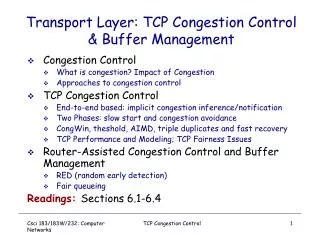
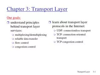
NS-2 LAB: TCP/IP Congestion control. Miriam Allalouf. 2005-2006 - Semester A. Networks Design Course Datagram Networks. Network Layer Service Model

E N D
NS-2 LAB: TCP/IP Congestion control Miriam Allalouf 2005-2006 - Semester A
Networks Design Course Datagram Networks Network Layer Service Model The transport layer relies on the services of the network layer : communication services between hosts. Router’s role is to “switch” packets between input port to the output port. Which services can be expected from the Network Layer? Is it reliable? Can the transport layer count on the network layer to deliver the packets to the destination? When multiple packets are sent, will they be delivered to the transport layer in the receiving host in the same order they were sent? Amount time between two sends equal to the amount time between two receives? Will be any congestion indication of the network? What is the abstract view of the channel connecting the transport layer in the sending and the receiving end points?
Networks Design Course Datagram Networks Best-effort serviceis the only service model provided by Internet. No guarantee for preserving timing between packets No guarantee of order keeping No guarantee of transmitted packets eventual delivery Network that delivered no packets to the destination would satisfy the definition of best-effort delivery service. IsBest-effort serviceequivalent tono service at all?
Networks Design Course Datagram Networks No service at all? Or What the advantages? Minimal requirementson the network layer easier to interconnect networkswith very different link-layer technologies:satellite, Ethernet, fiber, or radio use different transmission rates and loss characteristics. The Internet grew out of the need to connect computers together. Sophisticated end-system devicesimplement any additional functionality and new application-level network services at a higher layer. applications such as e-mail, the Web, and even a network-layer-centric service such as the DNS are implemented in hosts (servers) at the edge of the network. Simple new services addition: by attaching a host to the network and defining a new higher-layer protocol (such as HTTP) Fast adoption of WWW to the Internet.
full duplex data: bi-directional data flow in same connection MSS: maximum segment size connection-oriented: handshaking (exchange of control msgs) init’s sender, receiver state before data exchange flow controlled: sender will not overwhelm receiver point-to-point: one sender, one receiver reliable, in-order byte stream: no “message boundaries” pipelined: TCP congestion and flow control set window size TCP: OverviewRFCs: 793, 1122, 1323, 2018, 2581
32 bits source port # dest port # sequence number acknowledgement number head len not used rcvr window size U A P R S F checksum ptr urgent data Options (variable length) application data (variable length) TCP segment structure URG: urgent data (generally not used) counting by bytes of data (not segments!) ACK: ACK # valid PSH: push data now (generally not used) # bytes rcvr willing to accept RST, SYN, FIN: connection estab (setup, teardown commands) Internet checksum
Seq. #’s: byte stream “number” of first byte in segment’s data ACKs: seq # of next byte expected from other side cumulative ACK Q: how receiver handles out-of-order segments A: TCP spec doesn’t say, - up to implementor time TCP seq. #’s and ACKs Host B Host A User types ‘C’ Seq=42, ACK=79, data = ‘C’ host ACKs receipt of ‘C’, echoes back ‘C’ Seq=79, ACK=43, data = ‘C’ host ACKs receipt of echoed ‘C’ Seq=43, ACK=80 simple telnet scenario
At TCP Receiver: TCP ACK generation[RFC 1122, RFC 2581] TCP Receiver action delayed ACK. Wait up to 500ms for next segment. If no next segment, send ACK immediately send single cumulative ACK send duplicate ACK, indicating seq. # of next expected byte immediate ACK if segment starts at lower end of gap Event in-order segment arrival, no gaps, everything else already ACKed in-order segment arrival, no gaps, one delayed ACK pending out-of-order segment arrival higher-than-expect seq. # gap detected arrival of segment that partially or completely fills gap
Host A Host B Seq=92, 8 bytes data ACK=100 timeout X loss Seq=92, 8 bytes data ACK=100 time time lost ACK scenario TCP: retransmission scenarios Host A Host B Seq=92, 8 bytes data Seq=100, 20 bytes data Seq=92 timeout ACK=100 ACK=120 Seq=100 timeout Seq=92, 8 bytes data ACK=120 premature timeout, cumulative ACKs
Q: how to set TCP timeout value? longer than RTT note: RTT will vary too short: premature timeout unnecessary retransmissions too long: slow reaction to segment loss Q: how to estimate RTT? SampleRTT: measured time from segment transmission until ACK receipt ignore retransmissions, cumulatively ACKed segments SampleRTT will vary, want estimated RTT “smoother” use several recent measurements, not just current SampleRTT TCP Round Trip Time and Timeout
Setting the timeout EstimtedRTT plus “safety margin” large variation in EstimatedRTT -> larger safety margin TCP Round Trip Time and Timeout EstimatedRTT = (1-x)*EstimatedRTT + x*SampleRTT • Exponential weighted moving average • influence of given sample decreases exponentially fast • typical value of x: 0.125 (1/8) Timeout = EstimatedRTT + 4*Deviation Deviation = (1-x)*Deviation + x*|SampleRTT-EstimatedRTT|
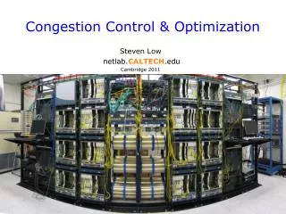
Congestion: informally: “too many sources sending too much data too fast for network to handle” different from flow control! manifestations: lost packets (buffer overflow at routers) long delays (queueing in router buffers) a top-10 problem! Principles of Congestion Control
two senders, two receivers one router, infinite buffers no retransmission large delays when congested maximum achievable throughput Causes/costs of congestion: scenario 1
one router, finite buffers sender retransmission of lost packet Causes/costs of congestion: scenario 2
always: (goodput) “perfect” retransmission only when loss: retransmission of delayed (not lost) packet makes larger (than perfect case) for same l l l > = l l l in in in out out out Causes/costs of congestion: scenario 2 “costs” of congestion: • more work (retrans) for given “goodput” • unneeded retransmissions: link carries multiple copies of pkt
four senders multihop paths timeout/retransmit l l in in Causes/costs of congestion: scenario 3 Q:what happens as and increase ?
Causes/costs of congestion: scenario 3 Another “cost” of congestion: • when packet dropped, any “upstream transmission capacity used for that packet was wasted!
End-end congestion control: no explicit feedback from network congestion inferred from end-system observed loss, delay approach taken by TCP Network-assisted congestion control: routers provide feedback to end systems single bit indicating congestion (SNA, DECbit, TCP/IP ECN, ATM) explicit rate sender should send at Approaches towards congestion control Two broad approaches towards congestion control:
end-end control (no network assistance) transmission rate limited by congestion window size, Congwin, over segments: w * MSS throughput = Bytes/sec RTT TCP Congestion Control Congwin • w segments, each with MSS bytes sent in one RTT:
Adjust Congestion window sending rate adjustment Slow Acks (low link or high delay) Slow cwnd Increase Fast Acks Fast cwnd Increase TCP Self-clocking
two “phases” slow start congestion avoidance important variables: Congwinbased on the perceived level of congestion. The Host receives indications of internal congestion threshold: defines threshold between two slow start phase, congestion control phase “probing” for usable bandwidth: ideally: transmit as fast as possible (Congwin as large as possible) without loss increaseCongwin until loss (congestion) loss: decreaseCongwin, then begin probing (increasing) again TCP congestion control:
exponential increase (per RTT) in window size (not so slow!) loss event: timeout (Tahoe TCP) and/or or three duplicate ACKs (Reno TCP) Slowstart algorithm time TCP Slowstart Host A Host B one segment RTT initialize: Congwin = 1 for (each segment ACKed) Congwin++ until (loss event OR CongWin > threshold) two segments four segments
TCP Congestion Avoidance Congestion avoidance /* slowstart is over */ /* Congwin > threshold */ Until (loss event) { every w segments ACKed: Congwin++ } threshold = Congwin/2 Congwin = 1 perform slowstart Reno Tahoe 1 1: TCP Reno skips slowstart (fast recovery) after three duplicate ACKs
Additive Increase is a reaction to perceived available capacity. Linear Increase basic idea: For each “cwnd’s worth” of packets sent, increase cwnd by 1 packet. In practice, cwnd is incremented fractionally for each arriving ACK. TCP congestion avoidance: AIMD:additive increase, multiplicative decrease increase window by 1 per RTT decrease window by factor of 2 on loss event Additive Increase AIMD increment = MSS x (MSS /cwnd) cwnd = cwnd + increment
Fast Retransmit • Coarse timeouts remained a problem, and Fast retransmit was added with TCP Tahoe. • Since the receiver responds every time a packet arrives, this implies the sender will see duplicate ACKs. Basic Idea:: use duplicate ACKs to signal lost packet. Fast Retransmit Upon receipt of three duplicate ACKs, the TCP Sender retransmits the lost packet.
Fast Retransmit • Generally, fast retransmit eliminates abouthalf the coarse-grain timeouts. • This yields roughly a 20% improvement in throughput. • Note – fast retransmit does not eliminate all the timeouts due to small window sizes at the source.
Fast Recovery • Fast recovery was added with TCP Reno. • Basic idea:: When fast retransmit detects three duplicate ACKs, start the recovery process from congestion avoidance region and use ACKs in the pipe to pace the sending of packets. Fast Recovery After Fast Retransmit, half cwnd and commence recovery from this point using linear additive increase ‘primed’ by left over ACKs in pipe.
Fairness goal: if N TCP sessions share same bottleneck link, each should get 1/N of link capacity TCP Fairness TCP connection 1 bottleneck router capacity R TCP connection 2
Two competing sessions: Additive increase gives slope of 1, as throughout increases multiplicative decrease decreases throughput proportionally Why is TCP fair? equal bandwidth share R loss: decrease window by factor of 2 congestion avoidance: additive increase Connection 2 throughput loss: decrease window by factor of 2 congestion avoidance: additive increase Connection 1 throughput R
TCP strains Tahoe Reno Vegas
Q:How long does it take to receive an object from a Web server after sending a request? TCP connection establishment data transfer delay Notation, assumptions: Assume one link between client and server of rate R Assume: fixed congestion window, W segments S: MSS (bits) O: object size (bits) no retransmissions (no loss, no corruption) TCP latency modeling Two cases to consider: • WS/R > RTT + S/R: ACK for first segment in window returns before window’s worth of data sent • WS/R < RTT + S/R: wait for ACK after sending window’s worth of data sent
TCP latency Modeling K:= O/WS Case 2: latency = 2RTT + O/R + (K-1)[S/R + RTT - WS/R] Case 1: latency = 2RTT + O/R
TCP Latency Modeling: Slow Start • Now suppose window grows according to slow start. • Will show that the latency of one object of size O is: where P is the number of times TCP stalls at server: - where Q is the number of times the server would stall if the object were of infinite size. - and K is the number of windows that cover the object.
TCP Latency Modeling: Slow Start (cont.) Example: O/S = 15 segments K = 4 windows Q = 2 P = min{K-1,Q} = 2 Server stalls P=2 times.
receiver: explicitly informs sender of (dynamically changing) amount of free buffer space RcvWindow field in TCP segment sender: keeps the amount of transmitted, unACKed data less than most recently received RcvWindow flow control TCP Flow Control sender won’t overrun receiver’s buffers by transmitting too much, too fast RcvBuffer= size or TCP Receive Buffer RcvWindow = amount of spare room in Buffer receiver buffering
Recall:TCP sender, receiver establish “connection” before exchanging data segments initialize TCP variables: seq. #s buffers, flow control info (e.g. RcvWindow) client: connection initiator Socket clientSocket = new Socket("hostname","port number"); server: contacted by client Socket connectionSocket = welcomeSocket.accept(); Three way handshake: Step 1:client sends TCP SYN control segment to server specifies initial seq # Step 2:server receives SYN, replies with SYNACK control segment ACKs received SYN allocates buffers specifies server-to-receiver initial seq. # Step 3:client sends ACK and data. TCP Connection Management
Closing a connection: client closes socket:clientSocket.close(); Step 1:client end system sends TCP FIN control segment to server. Step 2:server receives FIN, replies with ACK. Closes connection, sends FIN. client server close FIN ACK close FIN ACK timed wait closed TCP Connection Management (cont.)
Step 3:client receives FIN, replies with ACK. Enters “timed wait” - will respond with ACK to received FINs Step 4:server, receives ACK. Connection closed. Note:with small modification, can handly simultaneous FINs. TCP Connection Management (cont.) client server closing FIN ACK closing FIN ACK timed wait closed closed
TCP Connection Management (cont) TCP server lifecycle TCP client lifecycle
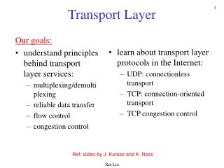
principles behind transport layer services: multiplexing/demultiplexing reliable data transfer flow control congestion control instantiation and implementation in the Internet UDP TCP Summary
Q mng : Packet Dropping : Tail Drop • Tail Drop –packets are dropped when the queue is full causes the Global Synch. problem with TCP Queue Utilization 100% Time Tail Drop
Packet Dropping : RED • Proposed by Sally Floyd and Van Jacobson in the early 1990s • packets are dropped randomly prior to periods of high congestion, which signals the packet source to decrease the transmission rate • distributes losses over time
RED - Implementation • Drop probability is based on min_threshold, max_threshold, and mark probability denominator. • When the average queue depth is above the minimum threshold, RED starts dropping packets. The rate of packet drop increases linearly as the average queue size increases until the average queue size reaches the maximum threshold. • When the average queue size is above the maximum threshold, all packets are dropped.
RED (cont.) Buffer occupancy calculation Average Queue Size – Weighted Exponential Moving Average 1 drop prob. … Max Prob av. queue size 0 min max
GRED Gentle RED Buffer occupancy calculation Average Queue Size – Weighted Exponential Moving Average 1 drop prob. … Max Prob av. queue size 0 min max 2*max