Download
1 / 27
280 likes | 481 Views
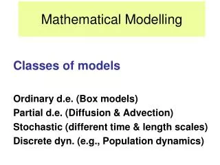
Mathematical Modelling. Classes of models Ordinary d.e. (Box models) Partial d.e. (Diffusion & Advection) Stochastic (different time & length scales) Discrete dyn. (e.g., Population dynamics). Liouville equation. d/dt x = A(x) d/d t r( x,t ) = - d/d x ( A( x ) . r( x,t) ). t.

E N D
Mathematical Modelling Classes of models Ordinary d.e. (Box models) Partial d.e. (Diffusion & Advection) Stochastic (different time & length scales) Discrete dyn. (e.g., Population dynamics)
Liouville equation d/dt x = A(x) d/dt r(x,t) = - d/dx(A(x) . r(x,t)) t
Liouville equation Governs the evolution of ρ(p,q;t) in time t # particles is the integral over phase space Liouville's theorem can be written F= dp/dt p/m=dx/dt
Brownian Motion Einstein,Orstein, Uhlenbeck, Wiener, Fokker, Planck et al. dx/dt = f(x) + g(x) dw/dt
Brownian motion is the random movement of particles, caused by their bombardment on all sides by bigger molecules. This motion can be seen in the behavior of pollen grains placed in a glass of water Because this motion often drives the interaction of time and spatial scales, it is important in several fields.
Following an idea of Hasselmann one can divide the climate dynamics into two parts. These two parts are the slowly changing climate part and rapidly changing weather part. The weather part can be modeled by a stochastic process such as white noise
Following an idea of Hasselmann one can divide the climate dynamics into two parts. These two parts are the slowly changing climate part and rapidly changing weather part. The weather part can be modeled by a stochastic process such as white noise
Langevin equation • In statistical physics, a Langevin equation is a stochastic differential equation describing Brownian motion in a potential. • The first Langevin equations: potential is constant, so that the acceleration of a Brownian particle of mass m is expressed as the sum of a viscous force which is proportional to the particles velocity (Stokes' law), a noise term representing the effect of a continuous series of collisions with the atoms of the underlying fluid (systematic interaction force due to the intermolecular interactions) Force Friction Noise
Relationship with Stochastic Differential Equations dX = μ(X,t)dt + σ(X,t)dB where X is the state and B is a standard M-dimensional Brownian motion. probability density of the state X of is given by the Fokker-Planck equation drift term diffusion
Fokker-Planck equation • The Fokker-Planck equation describes the time evolution of the probability density function of position and velocity of a particle. A standard scalar Brownian motion is generated by the stochastic differential equation dXt = dBt, Now the drift term is zero and diffusion coefficient is 1/2 and thus the corresponding Fokker-Planck equation is which is the simplest form of diffusion equation.
Markov Chains • A Markov chain is characterized by the conditional distribution • which is called the transition probability of the process. This is sometimes called the "one-step" transition probability. If the state space is finite, the transition probability distribution can be represented as a matrix, called the transition matrix, with the (i, j)'th element equal to
Master equation • In physics, a master equation is a phenomenological first-order differential equation describing the time-evolution of the probability of a system to occupy each one of a discreteset of states: • where Pk is the probability for the system to be in the state k, while the matrix is filled with a grid of transition-rate constants. • Note that • (i.e. probability is conserved), so the equation may also be written: • If the matrix is symmetric, ie all the microscopic transition dynamics are state-reversible so • this gives:
t t+dt n+1 n n-1
Difference Equations • Logistic Map • Chaotic dynamics was made popular by the computer experiments of Robert May and Mitchell Feigenbaum • The remarkable feature of the logistic map is in the simplicity of its form (quadratic) and the complexity of its dynamics. It is the simplest model that shows chaos. • The logistic map is the simplest model in population dynamics that incorporates the effects of both birth and death rates. It is given by the formula • xn+1 = b*xn*(1-xn) where the function f is called the logistic mapping and the parameter b models the effective growth rate. The population size is defined relative to the maximum population size the ecosystem can sustain and is therefore a number between 0 and 1. The parameter b is also restricted between 0 and 4 to keep the system bounded and therefore the model to make physical sense.
Fix points • How calculate? • x = b x (1-x) • Solving this equation gives two values x = 0 and x = 1 - 1/b.
Limit Cycles: Graphical method • 2 period limit cycle of the logistic equation can be thought of as the fixed point of the two composition of the logistic equation. • An m period limit cycle of the logistic equation can be thought of as the fixed point of the m composition of the logistic equation. • The 2 period limit cycle implies that xa = f ( xb ) and xb = f ( xa ). • Substituting the second equation in the first: xa = f ( f ( xa )) = f2( xa ). • Find the 2 period limit cycle: we look for the intersection of the diagonal line with the graph of the second composition of the logistic equation. • It can be seen that the green curve doesn't intersect the diagonal line for the first two plots and it does for b = 3.2 and 3.52.
STABILITY OF FIXED POINTS AND LIMIT CYCLES • examine the local behavior of the map in the vicinity of the fixed point or the limit cycle. The first derivative of the logistic equation is given by f' ( x ) = b (1 - 2*x) which is the slope of the parabola at point x. • To find the stability of the fixed point, we evaluate the slope at the fixed point and the following conditions characterize the behavior of the fixed point: | f' ( x ) | < 1 attracting and stable f' ( x ) = 0 super-stable | f' ( x ) | > 1 repelling and unstable | f' ( x ) | = 1 neutral
Stability of m period limit cycle • we evaluate the slope of fm( x ) Using the chain rule for differentiation, the above condition can be reduced to the evaluation of the expression • | f'( x1 ) × f'( x2 ) × ... , f'( xm ) |