Download
1 / 33
690 likes | 1.36k Views
Groundwater Modeling - 1. Groundwater Hydraulics Daene C. McKinney. Models …?. Input (Explanatory Variable). Precipitation. Soil Characteristics. Model (Represents the Phenomena). ET. Evaporation. Infiltration. Output (Results – Response variable) . Run off.

E N D
Groundwater Modeling - 1 Groundwater Hydraulics Daene C. McKinney
Models …? Input (Explanatory Variable) Precipitation Soil Characteristics Model (Represents the Phenomena) ET Evaporation Infiltration Output (Results – Response variable) Run off
Models and more models … Hydrologic Simulation Simulation Model Optimization Model Input (Explanatory Variable) Inflow Data Inflow Data Precip. & Soil Charact. Model (Phenomena) Basin Water Allocation Policy Basin Objectives and Constraints Mimic Physics of the Basin Output (Results) Response to the Policy Optimum Policy Runoff Source for Input data of other models Predict Response to given design/policy Identify optimal design/policy
Problem identification and description Model conceptualization Data Model development Model calibration & parameter estimation Model verification & sensitivity analysis Model Documentation Model application Present results Modeling Process 1 • Problem identification (1) • Important elements to be modeled • Relations and interactions between them • Degree of accuracy • Conceptualization and development (2 – 3) • Mathematical description • Type of model • Numerical method - computer code • Grid, boundary & initial conditions • Calibration (4) • Estimate model parameters • Model outputs compared with actual outputs • Parameters adjusted until the values agree • Verification (4) • Independent set of input data used • Results compared with measured outputs 2 3 4 5 6 7
Tools to Solve Groundwater Problems • Physical and analog methods • Some of the first methods used. • Analytical methods • What we have been discussing so far • Difficult for irregular boundaries, different boundary conditions, heterogeneous and anisotropic properties, multiple phases, nonlinearities • Numerical methods • Transform PDEs governing flow of groundwater into a system of ODEs or algebraic equations for solution
Conceptual Model • Descriptive representation of groundwater system incorporating interpretation of geological & hydrological conditions • What processes are important to model? • What are the boundaries? • What parameter values are available? • What parameter values must be collected?
What Do We Really Want To Solve? • Horizontal flow in a leaky confined aquifer • Governing Equations • Boundary Conditions • Initial conditions Flux Leakage Source/Sink Storage Ground surface Head in confined aquifer Confining Layer h Qx Confined aquifer b z y K x Bedrock
Finite Difference Method • Finite-difference method • Replace derivatives in governing equations with Taylor series approximations • Generates set of algebraic equations to solve 1st derivatives
Taylor Series • Taylor series expansion of h(x) at a point x+Dx close to x • If we truncate the series after the nth term, the error will be
First Derivative - Forward • Consider the forward Taylor series expansion of a function h(x) near a point x • Solve for 1st derivative
First Derivative - Backward • Consider the backward Taylor series expansion of a function f(x) near a point x • Solve for 1st derivative
Finite Difference Approximations i 1st Derivative (Backward) 1st Derivative (Forward)
y, j Mesh Domain i,j+1 D y i-1,j i,j i+1,j Node point i,j-1 x, i D x Grids and Discretrization • Discretization process • Grid defined to cover domain • Goal - predict values of head at node points of mesh • Determine effects of pumping • Flow from a river, etc • Finite Difference method • Popular due to simplicity • Attractive for simple geometry Grid cell
Three-Dimensional Grids • An aquifer system is divided into rectangular blocks by a grid. • The grid is organized by rows (i), columns (j), and layers (k), and each block is called a "cell" • Types of Layers • Confined • Unconfined • Convertible j, columns i, rows k, layers Layers can be different materials
1-D Confined Aquifer Flow Ground surface • Homogeneous, isotropic, 1-D, confined flow • Governing equation • Initial Condition • Boundary Conditions Confining Layer hA Aquifer Node Dx hB b z y x i = 0 1 2 3 4 5 6 7 8 9 10 Grid Cell
Derivative Approximations • Need 2nd derivative WRT x
Derivative Approximations • Governing Equation • 2nd derivative WRT x • Need 1st derivative WRT t Which one to use? Forward Backward
Time Derivative • Explicit • Use all the information at the previous time step to compute the value at this time step. • Proceed point by point through the domain. • Implicit • Use information from one point at the previous time step to compute the value at all points of this time step. • Solve for all points in domain simultaneously.
Explicit Method • Use all the information at the previous time step to compute the value at this time step. • Proceed point by point through the domain. • Can be unstable for large time steps. FD Approx. Forward
Explicit Method l+1 time level unknown l time level known
1-D Confined Aquifer Flow Ground surface • Initial Condition • Boundary Conditions Confining Layer hA Aquifer Node Dx hB b z y x Dx= 1 m L = 10 m T=bK= 0.75 m2/d S= 0.02 i = 0 1 2 3 4 5 6 7 8 9 10 Grid Cell L
Explicit Method Ground surface Confining Layer hA Aquifer Node Dx hB b i = 0 1 2 3 4 5 6 7 8 9 10 Consider: r = 0.48 r = 0.52 Grid Cell Dx= 1 m L = 10 m T = 0.75 m2/d S= 0.02
What’s Going On Here? Ground surface • At time t = 0 no flow • At time t > 0 flow • Water released from storage in a cell over time Dt • Water flowing out of cell over interval Dt Confining Layer hA Aquifer Dx hB b Dx i = 0 1 2 … i-1 i i+1 … 8 9 10 Grid Cell i r > 0.5 Tme interval is too large Cell doesn’t contain enough water Causes instability
Implicit Method • Use information from one point at the previous time step to compute the value at all points of this time step. • Solve for all points in domain simultaneously. • Inherently stable FD Approx. Backward
Implicit Method l+1 time level unknown l time level known
2-D Steady-State Flow • General Equation • Homogeneous, isotropic aquifer, no well • Equal spacing (average of surrounding cells) Node No. Unknown heads Known heads
2-D Heterogeneous Anisotropic Flow Txand Tyare transmissivities in the x and y directions
2-D Heterogeneous Anisotropic Flow • Harmonic average transmissivity
MODFLOW • USGS supported mathematical model • Uses finite-difference method • Several versions available • MODFLOW 88, 96, 2000, 2005 (water.usgs.gov/nrp/gwsoftware/modflow.html) • Graphical user interfaces for MODFLOW: • GWV(www.groundwater-vistas.com) • GMS(www.ems-i.com) • PMWIN(www.ifu.ethz.ch/publications/software/pmwin/index_EN) • Each includes MODFLOW code
What Can MODFLOW Simulate? • Unconfined and confined aquifers • Faults and other barriers • Fine-grained confining units and interbeds • Confining unit - Ground-water flow and storage changes • River – aquifer water exchange • Discharge of water from drains and springs • Ephemeral stream - aquifer water exchange • Reservoir - aquifer water exchange • Recharge from precipitation and irrigation • Evapotranspiration • Withdrawal or recharge wells • Seawater intrusion