Download
1 / 35
350 likes | 356 Views
Wireless Communication Issues in Sensor Networks. Alec Woo UC Berkeley October 2 nd , 2003. Theme. Explore underlying communication issues and their effects on high-level protocol design Single hop Zhao and Govindan, SenSys 2003 Extra: SCALE (Cerpa et al. CENS TR 2003)

E N D
Wireless Communication Issues in Sensor Networks Alec Woo UC Berkeley October 2nd, 2003
Theme • Explore underlying communication issues and their effects on high-level protocol design • Single hop • Zhao and Govindan, SenSys 2003 • Extra: SCALE (Cerpa et al. CENS TR 2003) • Network-level protocol • multi-hop routing for data collection. (Woo et al., SenSys 2003)
Motivation • Why do we care about all these details? • we will experience it! • if we want to implement our protocols • actual deployment decision
Roadmap • Single Hop packet loss characteristics • Core dimensions • Environment, distance, transmit power, temporal correlation, data rate, packet size • Services for High Level Protocols/Applications • Link estimation • Neighborhood management • Reliable Multihop Routing
Zhao’s Study • Hardware • Mica, RFM 433MHz • MAC • TinyOS Mac (CSMA) • Encoding • Manchester (1:2) • 4b/6b (1:1.5) • SECDED (1:3) • Environment • Indoor, Open Structure, Habitat Environment
Indoor is the Harshest • Linear topology over a hallway (0.5/0.25m spacing) • 40% of the links have quality < 70% • Lower transmit power • yields smaller tail distribution • SECDEC • significantly helps to lower the heavy tail
Packet Loss and Distance • Gray/Transitional Area • ranges from 20% to 50% of the communication range • Habitat has smaller communication range? • Other evidence (Cerpa et al., Woo et al.) • RFM: BAD RADIO??
ChipCon Radio (Cerpa et al.) Mica On Ceiling • Higher transmit power doesn’t eliminate transitional region • Range in (a) and (b) are the same? • Indoor RFM result is worst than that in Zhao’s work • cannot even see the effective region
Can better coding help? • SECDED is effective if start symbol is detected but does not increase “communication range” • Bit error rate (BER) is higher in transitional region • Missing start symbol is fatal • Better coding for start symbol?
Loss Variation (Cerpa et al.) • Variation over distance and over time • binomial approximation for variation over time? • Zhao shows that SECDED helps decrease the variation over distance (but very large SD here)
Packet Loss vs. Workload • Packet loss increases as network load increases • But what is the network load? • How many nodes are in range? • Not sure! • Is 0.5packets/s already in saturation? • Difficult to observe is it hidden node terminal
Packet Loss vs. RSSI • Low packet loss => good RSSI • But not vice versa • Too high a threshold limits number of links • Network partition??
Other Findings • Correlation of Packet Loss • correlation at the gray (transitional) region for indoor • Habitat: much less • Independent losses are reasonable • 50%-80% of the retransmissions are wasted • Neighbor = hear a node once • Asymmetric links are common • > 10% of link pairs have link quality difference > 50% • Cerpa et al. • Moving a little bit doesn’t help • Swap the two nodes, asymmetrical link swaps too • i.e. not due to the environment
Packet Size (Cerpa et al.) • Loss over distance is relatively the same for different packet size (25 bytes and 150 bytes) at different transmit power
Take Away • Who to blame? • Radio? • Similar results found over RFM and ChipCon radio • Hardware calibration! Yeah! • Base-band radio • Multi-path will remain unless spread-spectrum radio is used • But 802.11 is also not ideal (Decouto et al. Mobicom 03) • What is the effective communication range? • What does it mean when you deploy a network • What defines a neighbor? • Why study high density sensor network? • Break?
Roadmap • Single Hop packet loss characteristics • Core dimensions • Environment, distance, transmit power, temporal correlation, data rate, packet size • Services for High Level Protocols/Applications • Link estimation • Neighborhood management • Reliable multihop routing for data collection
Link Quality Estimation • Estimate rate of successful reception from neighboring nodes • RSSI may not work well • Neighbors exchange estimations to derive bi-directional link quality • 2 Techniques: Passive vs. Active • Key decision factor: broadcast medium • Passive: snoop on neighbor packets
What is a good Estimator? • For a given error bound and agility, • yields the most stable estimation • with the smallest memory footprint • and the simplest algorithm • Agility and stability are at odds with each other
Agility and Error Bound • Simulation worst case: 10% error ~ 100 packet time • Assuming IID Binomial model, by the central limit theorem • Worst case (p = 0.5) requires • 10% error with 90% confidence requires ~100 packet opportunities to learn • For example: at 30sec/packet • 50 minutes for 100 packets • forwarding traffic helps to reduce this time but potentially a long delay • Major disadvantage
Infer Packet Loss • Packet sequence number for inferring packet loss • Issue: cannot infer loss until hearing the next packet • E.g. dead node or mobility • Can infer losses based on time • Assume minimum data rate is known • Likely to be true in periodic data collection
WMEWMA Estimator • Compute an average success rate over time, T, and smoothes with an exponentially weighted moving average (EWMA) • Average calculation • Packet Received over T divided by • Max of • Number of packets expected over T • Number of packets sent over T suggested by sequence number • Tuning parameters: • T and history size of EWMA • Performance • Yields agile and stable estimations • Uses constant memory, and is very simple
Neighbor Table • Maintain link estimation statistics and routing information of each neighbor • How large should this table be? • O(cell density) * meta-data for each neighbor • Issue: • Density can be high but memory is limited • At high density, many links are poor or asymmetric • Question: • Can we use constant memory to maintain a set of good neighbors regardless of cell density?
Neighborhood Management • Question: when table becomes full, • should we add new neighbor? • If so, evict which old neighbor? • Neighbor Goodness • Basic one is link quality but it is unknown • Signal strength is a hint • Rely on frequency of packet reception • Assume periodic data packets or beacons • Similar to • frequency estimation of data streams, or • classical cache policy
Management Algorithm • When we hear a node, if • In table: increment a counter for this node • Not in table • Insert if table is not full • down-sample if table is full • If successful, insert only if some nodes can be evicted • Eviction: (FREQUENCY) • Decrement counter for each table entry • Nodes with counter = 0 can be evicted • Otherwise, all nodes stay in the table
Key Results • FREQUENCY algorithm can effectively • utilize 50% to 70% of the table space to maintain a set of good neighbors • while being adaptive to neighborhood changes • Routing simulation: • Neighbor goodness is augmented to avoid maintaining sibling nodes based on routing cost difference
Reliable Routing • 3 core components for Routing • Routing protocol • Neighbor table management • Link estimation • Example • Tree based routing for data collection • Reliable end-to-end packet delivery with minimum number of transmissions (link retransmissions) • Advocate stability • Simple
Design Issues • Shortest path alone yields poor end-to-end success rate • Multi-hop over bad links has exponential loss effect • Two approaches • SP over some link quality threshold • Minimum expected number of transmissions as routing cost • Route damping • New route is not evaluated on every route updates • Link failure detection using consecutive packet loss leads to instability • link quality characterization is better • Queuing Policy • Two queues • Fair allocation between forwarding and originating traffic • Cycles • Detection vs. loop-free
SP with Threshold • High threshold (e.g. 70%) fails to form a tree • Works fine in simulation! • link quality degrades when there is traffic • High threshold leads to network partition • Echo the observation made in Zhao’s work • Lower threshold (e.g. 40%) is also problematic • Tree prunes and rebuilds over time when traffic is high
MT • No predefine threshold is necessary • Captures both reliability and energy cost • Routing cost builds upon individual estimations along the path • Cost = hops + number of expected link retransmissions • if link quality = 100%, MT reduces to normal SP routing
Methodology • Graph analysis • Network simulation • Assuming packet loss are independent, following Binomial model • Empirical evaluation • On site connectivity vs. distance study • Find minimum transmit power • Transitional/gray area starts at average node distance
Findings (I) • Hop distribution and success rate • longer majority hop-count yields higher success • Hop distribution and distance • Evidence of long links, potentially reliable • Retransmissions are not too effective • MT yields ~80% success rate • packets delivered only experience 1 retransmission along the path • A maximum of 2 retransmission per hop can • Needs a maximum of 3 per hop to achieve over 90% end-to-end success rate
Findings (II) • Link failure detection with consecutive packet loss leads to instability • Stability and Congestion • link quality fluctuates at congestion period • creates global instability • BS can hear half the number of neighbors in the network even with a low power setting • MT metrics build upon link estimations are stable • No cycles are detected
Discussions (I) • Passive snooping • What are the assumptions for this to work? • Estimation takes too long • Can we infer from BER before FEC? (tricky)? • But missing start symbol is the major cause! • Neighborhood management argument • Do you buy it? • Stability • Do we care? • Congestion • How to avoid it? • Scheduled communication?
Discussions (II) • Can we define a hop? • One hop neighbor? • What is the averaged hop distance? • Deployment • What’s the expected hop-count? • What distance or transmit power should we use? • Overhead • Anecdotal setting of route update rate • Can it be adaptive?
Discussion (III) • Power • No address on power management • How does it work with scheduled communication which avoids overhearing? • Potentially run over low-power listening • What’s used in Great Duck Island • DSDV (Yarvis et al. ICPP Workshop 2002) • Different kinds of link estimation and routing cost • Do we need to prevent cycle like DSDV in a relatively static network? • N-to-N Routing?