Download
1 / 37
370 likes | 385 Views
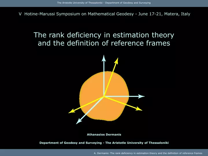
V Hotine-Marussi Symposium on Mathematical Geodesy - June 17-21, Matera, Italy. The rank deficiency in estimation theory and the definition of reference frames. Athanasios Dermanis Department of Geodesy and Surveying - The Aristotle University of Thessaloniki. Coordinates.

E N D
V Hotine-Marussi Symposium on Mathematical Geodesy - June 17-21, Matera, Italy The rank deficiency in estimation theory and the definition of reference frames Athanasios Dermanis Department of Geodesy and Surveying - The Aristotle University of Thessaloniki
Coordinates Field of local vector bases Relativity theory: Description of space-time: Description of local vectors - tensors:
Reference frame: Origin + 3 base vectors (orthonormal for convenience) Parallel translation of vector basis to any point (axiom of parallelism) Position vector concept: Cartesian coordinates = = components of position vector: Newtonian physics: Separation of space from time - Euclidean space model Description of local vectors - tensors: Description of space:
Reference frame: A modeling device for the provision of - a field of (parallel) local frames for local tensor representation, - a system of (cartesian) coordinates for the description of “places” (also curvilinear coordinates defined as functions of cartesian). A reference frame has no physical meaning and cannot be determined from observations. It must be established by introducing arbitrary conventions in the process of data analysis. Its use has the advantage of facilitating mathematical modeling of physical processes and the disadvantage of leading to equations with no unique solutions (rank deficient models)
Modeling: Simplification of natural processes andisolation of a part of nature in relation to a performed set of measurements corresponding to a set of observables . Errors: discrepancies accounting for effects of isolation and simplification. Parametric rank of physical system: Minimal number of parameters needed to describe the system (all other parameters can be expressed as functions of a describing set of parameters). Model parameters: observables & additional unknown parameters Model equations: equations of the form Examples: , (no unknowns ): Condition equations , (describing set ): Observation equations Modeling Physical system covered by observations: Set of all parameters that can be virtually expressed as functions of observables.
Use of m parameters x describing a system S' System covered by observations SS'with rank r<m S' S Question: When does a parameter q(x)S ? Or: is q(x) determinable from the observables? Answer: When it can be expressed as a function of y:q(x)=d(y)=d(f(x))! q=dofdeterminability condition Improper modelingy=f(x)(model without full rank) Geodetic network example: S= shape and size S' = shape, size and position y = angles and distances, x = coordinates Problem circumvention: Arbitrarily fix S'-S by d=m-r conditions c(x)=0 (minimal constraints) Geodetic network example: Use minimal constraints to introduce an arbitrary reference frame
= BLUE of : Uniformly unbiased ( ), linear ( ) with minimum mean square error ( ) “Stochastic” definition of estimability: is estimable when there exists a uniformly unbiased linear estimate of “Deterministic” condition of estimability: (linear version of determinability condition ) Estimable parameter = it can be expressed as function of the observables: Parameter estimability in rank-deficient linear models
BLUE of : where is any solution of the normal equations: No unique solution because has If , are two solutions of the normal equations then: Invariant estimates of observables! If is estimable: Invariant estimate! Invariance of observables and estimable quantities
Solutions of normal equations: Transformations leaving observables invariant: leave estimable quantities invariant: The geometry of the linear model
The geometry of the linear model To each yR(A) corresponds a solution space Sy parallel to the null space N(A)=S0 As y varies over R(A) the disjoint solution spaces Sy cover the whole space X They form a fibering of X
The geometry of the linear model To each yR(A) corresponds a solution space Sy parallel to the null space N(A)=S0 As y varies over R(A) the disjoint solution spaces Sy cover the whole space X They form a fibering of X
The geometry of the linear model To each yR(A) corresponds a solution space Sy parallel to the null space N(A)=S0 As y varies over R(A) the disjoint solution spaces Sy cover the whole space X They form a fibering of X
The geometry of the linear model To each yR(A) corresponds a solution space Sy parallel to the null space N(A)=S0 As y varies over R(A) the disjoint solution spaces Sy cover the whole space X They form a fibering of X
The geometry of the linear model To each yR(A) corresponds a solution space Sy parallel to the null space N(A)=S0 As y varies over R(A) the disjoint solution spaces Sy cover the whole space X They form a fibering of X
The geometry of the linear model To each yR(A) corresponds a solution space Sy parallel to the null space N(A)=S0 As y varies over R(A) the disjoint solution spaces Sy cover the whole space X They form a fibering of X
The geometry of the linear model To each yR(A) corresponds a solution space Sy parallel to the null space N(A)=S0 As y varies over R(A) the disjoint solution spaces Sy cover the whole space X They form a fibering of X
The geometry of the linear model Minimum norm solution If is a basis for : Inner constraints
Minimal constraints: The linear subspace is a section of the fibering of the solution spaces, i.e. it intersects each in a single element Solution for BLUE estimates: - Satisfying constraints and normal equations The geometry of the linear model
Trivial constraints: Can be applied a priori: Unique solution: Estimable !? The unknowns are estimable only if the trivial constraints are “true”, i.e. they have a valid physical meaning within the model! The same holds true for any minimal constraints ! Note the difference between formalestimability when are arbitrary and true estimability when are physically valid within the model! The peculiar character of trivial constraints
Trivial constraints: Origin at P1 x axis along P1P2 line x, y plane at P1 P2 P3 plane Physically meaningful trivial constraints in geodetic networks Angle and distance observations: shape and size determination For any point P: zP = distance of P from P1P2P3 plane yP = distance of projection of P on P1P2P3 plane from line P1P2 xP = distance of projection of P1 on P1P2 line from point P1P2 These are parameters relating only to the shape and size of the network, independent from its position and orientation and thus estimable parameters. Furthermore: The trivial constraints determine the reference frame in a deterministic way, independently of the uncertainties present in the stochastic estimates of network coordinates.
Space of observations Space of coordinates Space of observables: Every point y = = a particular network shape Coordinates corresponding to the same shape (different frames): Least-squares solutions: Transformations leaving observables invariant: leave estimable quantities invariant: The reference frame problem in geodetic networks: The nonlinear picture
The reference frame problem in geodetic networks: The nonlinear picture Space of observations Space of coordinates General form of transformations leaving observables (shape) invariant: Similarity transformation. s=0 Rigid transformation, R= orthogonal Transformation parameters:
The reference frame problem in geodetic networks: The nonlinear picture Space of observations Space of coordinates Fixing a point the parameters of the transformation may serve as a set of coordinates on
Basis of tangent space to at : The reference frame problem in geodetic networks: The nonlinear picture Space of observations Space of coordinates Fixing a point the parameters of the transformation may serve as a set of coordinates on Columns of the matrix of inner constraints :
The problem: Observations determine the shape at every epoch t Space of coordinates At the shape manifold Sy(t) select a frame x(t) in a smooth way A reference frame RF is a curve in X intersecting the manifolds Sy(t) at a single point x(t) for each t Starting from any frame RF0 an optimal frame RF can be computed by determining the relevant transformation parameters p from x0(t) to x(t) : Parallel frames RF and RF’: The evolution of the reference frame in time Open question: What is a optimal frame? Two parallel frames are dynamically equivalent. Thus the initial epoch reference frame x0(t) must be arbitrarily fixed !
A geodesic on the manifold A generalization of the Meissl ladder concept: A discrete Tisserand principle (vanishing relative angular momentum): The optimal (time evolution) of the reference frame The surveying discrete time practice: Use coordinates estimates of epoch tk-1 as approximate coordinates for the epoch tk . Best fit the frame of tk to the frame of tk-1 by applying inner constraints on xk=xk-xk-1. Build a Meissl ladder! Alternatives for continuous time: They are all equivalent and lead to a system of nonlinear ordinary differential equations to be satisfied by the parameters p(t) of transformation from a given to the optimal frame. Initial conditions (integration constants): Choice between equivalent parallel frames.
Introduction of an analytical time evolution model - Deformation linear in time Discrete Tisserand condition: Linearized form: Usual form for : Plus the standard inner constraints for corrections at the initial epoch The ITRF approach
Equations of rotational motion: =angular momentum, = torque where: rotation (angular velocity) vector matrix (tensor) of inertia relative angular momentum Reference frames in earth rotation theories Inertial frame: Terrestrial frame: In terrestrial frame: Liouville equations Euler geometric equations
Terrestrial frame origin: geocenter Axes of figure: diagonal inertia tensor - NOT USED Tisserand axes: vanishing relative angular momentum Simplified Liouville equations: Reference frames in earth rotation theories Terrestrial frame orientation: Simplification of rotation equations - 2 choices A family of parallel frames: Arbitrary choice of initial epoch orientation !
Geodetic frame: Discrete, its definition depends on the shape of the defining network. Tisserand frame: Continuous, its definition depends on mass distribution and motion for the whole earth. Connecting the geodetic network reference frame with the geophysical earth frame of rotation theory The connection between geodetic (ITRF) and Tisserand frame requires: - Estimation of the position of geocenter with respect to the geodetic frame from satellite geodetic techniques (gravity field also unknown) - Estimation of earth motion and density from surface (network) motions and geophysical data.
Estimability of geocenter position Problem unknowns: Coordinates and gravity field parameters Both depend on reference frame Coordinate transformation of a point P due to change of reference frame: Representation of unknown function V(P) (gravitational potential) in terms of basis functions involving coordinates: Induced transformation on function coefficients :
Estimability of geocenter coordinates The null space basis for coordinates : columns of from The null space basis for function coefficients : columns of from The combined null space: columns of Linearized model: Inner constraints: Estimability conditions for geocenter coordinates :
The null space for coordinates and unknown function coefficients Expand: We seek only: We need to realize the expansion: For curvilinear coordinates :
The null space for spherical harmonic coefficients Expand: Compute: where Required expansions for spherical harmonics: Translation: Rotation: Scale:
Transformation from ITRF coordinates x to estimates of Tisserand coordinates: Angular momentum and inertia matrix for each subnetwork DK: Plate rotation vector: Plate inertia matrix: ITRF to Tisserand frame rotation vector and matrix: weighted mean! determines one out of infinite parallel Tisserand frames ! Estimating the direction of the earth Tisserand axes Each plate PK is represented by a subnetwork DK - Assume rotation-only model for plates
This powerpoint presentation is available at: http://der.topo.auth.gr
See you in Thessaloniki ! 3rd Meeting of the International Gravity and Geoid Commission IAG - Section III August 26-30, 2002 Thessaloniki, Greece http://der.topo.auth.gr/gg2002