Download
1 / 35
350 likes | 540 Views
Modeling the HIV/AIDS Epidemic in Cuba. Presented by Raluca Amariei and Audrey Pereira 2005 PIMS Mathematical Biology Summer School. Outline. Introduction to HIV HIV in Cuba Models Analysis of Models Output of Model III Fitting Model III to Data Extensions to the Model Conclusions.

E N D
Modeling the HIV/AIDS Epidemic in Cuba Presented by Raluca Amariei and Audrey Pereira 2005 PIMS Mathematical Biology Summer School
Outline • Introduction to HIV • HIV in Cuba • Models • Analysis of Models • Output of Model III • Fitting Model III to Data • Extensions to the Model • Conclusions
HIV the Virus In 2000: • 36.1 million people living with HIV • 390 000 in the Caribbean region • Only 3230 cases in Cuba (Cuba's 0.03% infection rate is one of the lowest in the world) • HIV - human immunodeficiency virus that causes Acquired Immuno-Deficiency Syndrome • AIDS - weakness in the body's system that fights diseases (CD4+ cell percentage is less than 14% )
HIV in Cuba • National Programme on HIV/AIDS established by the Cuban government in 1983: • Testing blood donations • Hospital surveillance - screening of patients with other STD’s, pregnant women, other hospital patients • HIV screening for travellers to other countries
HIV in Cuba • HIV seropositives placed in sanatoriums • Partner Notification Programme – contact tracing and screening of sexual partners • Increase in the HIV cases due to growth of tourism after 1996 • Negative impact of US Embargo on Cuban Health Services
Model I - Parameters • b = birth rate; d = death rate • τ1 = probability of acquiring HIV when in contact with an HIV+ • τ2 = probability of acquiring HIV when in contact with an AIDS sufferer • k = conversion rate of HIV to AIDS (incubation period = 9 yrs) • d’ = death rate for AIDS sufferers b S d τ1 τ2 d’ H A D k d d
Model I Equations: (1) S’ = b(S+H+A) - τ1SH - τ2SA - dS (2) H’ = τ1SH + τ2SA - kH - dH (3) A’ = kH – d’A – dA (4) D’ = d’A No deaths from AIDS N = S + H + A = constant (b=d) → N’ = 0 → S’+H’+A’ = 0 →d’=0
Analysis of Model I • Equilibrium Points: From (3): A = kH/d In (2), case (i) H = 0 → A = 0 → S = N Disease Free Equilibrium is: DFE = (N, 0, 0)
Analysis of Model I In (2), case (ii) H ≠ 0 divide (2) by H: τ1S + τ2kSH/d - k - d = 0 → S* = (k+d)/(τ1+τ2k/d)
Analysis of Model I Plug (2) and (3) in (1): H* = (d-b)S/(b+bk/d-k-d) But b=d → H* = 0. Contradiction. → there is noendemic equilibrium
Stability • Jacobian Matrix: J =
Stability of the DFE: • Jacobian Matrix at the DFE=(N, 0, 0): J(DFE) =
Stability of the DFE: Eigenvalues One eigenvalue is 0: λ1 = 0 The other two are found using the 2x2 matrix: J’ = Characteristic polynomial is λ2 – tr(J’) λ + det(J’) = 0
Stability of the DFE: Eigenvalues: λ2 + (k+2d-τ1N)λ + d(k+d-τ1N)-kτ2N = 0 By Routh-Hurwicz Criterion (n=2), roots have negative real part when: k+2d-τ1N > 0 d(k+d-τ1N)-kτ2N > 0 ↔ DFE is locally asymptotically stable ↔ kτ2N / [d(k+d-τ1N)] < 1 R0 – the number of new infections determined by one infective introduced in a susceptible population R0
Model II Assumptions: N not constant → b ≠ d. Let λ = b – d N’ = (b - d)N = λN → N(t) = N(0)eλt Let n(t) = e-λtN(t)= e-λt ( S(t) + H(t) + A(t) ) Apply the transformations for all classes: s(t) = e-λtS(t) h(t) = e-λtH(t) a(t) = e-λtA(t) d(t) = e-λtD(t) And then n(t) = s(t) + h(t) + a(t)
Model II Transformation of H(t): h(t) = e-λtH(t) h’(t) = -λe-λtH(t) + e-λtH’(t) = -λh(t) + e-λt(τ1SH/N + τ2SA/N - kH - dH) = -bh - kh+ τ1sh/n + τ2sa/n • Using standard incidence H/N and S/N
Model II s’(t) = bh + ba - τ1sh/n - τ2sa/n h’(t) = - bh - kh + τ1sh/n + τ2sa/n a’(t) = - ba + kh - d’a Equations: n = s + h + a n’ = s’ + h’ + a’ n’ = - d’a n(t) → 0
Model II Equilibrium Points: • Still no endemic equilibrium (obtain contradiction) • Disease Free Equilibrium: DFE = (n*, 0, 0)
Model II Stability of the DFE=(n*, 0, 0): One eigenvalue λ1 = 0 and λ2 + (2b+k+d’–τ1)λ + (b+d’)(b+k-τ1)-kτ2 = 0 Routh-Hurwicz Criterion: (2b+k+d’–τ2 ) > 0 (b+d’)(b+k-τ1)-kτ2 > 0
Model II Therefore the DFE is stable when: (b+d’)(b+k-τ1)-kτ2 > 0 ↕ kτ2 /[(b+d’)(b+k-τ1)] < 1 R0 Comparison: (I) R0 = kτ2N / [b(k+b-τ1N)] (II) R0 = kτ2 / [(b+d’)(b+k-τ1)]
Model III Equations: (1) S’ = b(S+H+A) - τ1SH - τ2SA - dS (2) H’ = τ1SH + τ2SA - kH - dH (3) A’ = kH – d’A – dA (3) D’ = d’A Assumptions: N not constant → b ≠ d
Model III – Equilibria Endemic Equilibrium: H ≠ 0: From (3): A = kH/(d+d’) From (2): S = (k+d)/[τ1+τ2k/(d+d’)] Substitute in (1): H = (b-d)(k+d)/[(k+d-b-bk/(d+d’))(τ1+τ2k/(d+d’))] N not constant → no DFE
Model III Endemic Equilibrium: S* = (k+d)/[τ1+τ2k/(d+d’)] H* = (b-d)(k+d)/[(k+d-b-bk/(d+d’))(τ1+τ2k/(d+d’))] A* = kH*/(d+d’)
Model III: Stability of the Endemic Equilibrium Jacobian matrix written in Maple:
Model III: Stability of the Endemic Equilibrium Characteristic Polynomial given by Maple: x3 + ax2 + bx + c = 0 By Routh-Hurwicz Criterion (n=3), the endemic equilibrium is locally asymptotically stable when: a > 0, c > 0, ab > c
Data • Given data: • 1986-2000 • New HIV Cases • New Aids Cases • Deaths each year from AIDS
Fitting Model III to Data HIV Cases Deaths from AIDS Legend: Given data Solution Curves of Model III AIDS Cases
Fitting Model III to Data Parameters: b = 0.114 d = 0.073 τ1= 0.15x10⁻⁵ τ2 = 0.12x10⁻⁶ k = 0.165 d’ = 0.195
Conclusions I: Problems • Time Limitations • In simulations • In model development • Discrete Model? Stochastic Model?
Extensions to the Model • Suggestions for improvement: • Females / Males • Heterosexual / Homosexual (it started as a heterosexual disease, now 90% of seropositives are males) • Exposed class - not infectious right away • Include the people infected but unaware (an estimate of 20-30% of the HIV asymptomatic carriers have not been detected) • Different number of sexual partners (differentiation between probabilities of transmission)
Extensions to the Model • Suggestions for improvement: S E Hu F Ha A D M Approximately 18 equations... Mh
Conclusions: • 3,200 HIV cases in Cuba Comparison with Canada in 2003: • In Ontario - approximately same population as Cuba (12 million), but 23,863 HIV cases • 12,156 HIV cases in Quebec (7 million) • 11,346 HIV cases in British Columbia (3 million) • 5 times more cases in QC • 8 times more cases in ON • 13 times more cases in BC
References 1. H de Arazoza and R. Lounes 2002. A non-linear model for a sexually transmitted disease with contact tracing. IMA J Math Appl Med Biol. Sep;19(3):221-34. 2. R. Lounes and H. de Arazoza 1999. A two-type model for the Cuban national programme on HIV/AIDS. IMA J Math Appl Med Biol. Jun;16(2):143-54. 3. Y.H Hsieh, de Arazoza H., Lee S.M., Chen C.W. Estimating the number of Cubans infected sexually by human immunodeficiency virus using contact tracing data. Int J Epidemiol. Jun;31(3):679-83. 4. BBC: Cuba leads the way in HIV fight. 2003 M. Bentley. http://news.bbc.co.uk/1/hi/in_depth/sci_tech/2003/denver_2003/2770631.stm