Download
1 / 29
290 likes | 405 Views
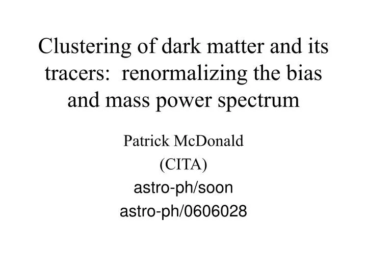
Clustering of dark matter and its tracers: renormalizing the bias and mass power spectrum. Patrick McDonald (CITA) astro-ph/soon astro-ph/0606028. Observational Motivation:. Non-linear power spectrum. Galaxies/BAO Lya forest Cosmic shear clusters/SZ 21 cm(?)

E N D
Clustering of dark matter and its tracers: renormalizing the bias and mass power spectrum Patrick McDonald (CITA) astro-ph/soon astro-ph/0606028
Observational Motivation: Non-linear power spectrum • Galaxies/BAO • Lya forest • Cosmic shear • clusters/SZ • 21 cm(?) • Red non-linear curves from Smith et al. simulation fits, not perfectly accurate
Best short-term motivation: Galaxy clustering(Padmanabhan et al. 2006, SDSS LRGs, photo-z) • Baryonic accoustic oscillations (dark energy) • Shape of power spectrum (omega_m, neutrinos) • Non-linearities • Bias • (Redshift-space distortions)
Why not just use simulations? • Incredibly slow and painful, to the point where no one has pushed through a complete, accurate (well-tested) mass power spectrum result, even though everyone knows it is just a matter of effort to do it. • Galaxies, and other observable tracers of mass, can’t be simulated rigorously, so it is useful to use a variety of calculational methods to get an indication of the robustness of results (plus, again, speed).
General idea of renormalization • Not just absorbing infinite quantities into parameters of a Lagrangian (or integrating out degrees of freedom). • Quantities to be renormalized can be any not-directly-observable numbers in the problem, including those specifying the initial/boundary conditions (don’t have to be infinite). • In the present context it is probably better to think of it as a rearrangement of a (supposedly) perturbative series to improve its convergence, although this is not explicit in the RG calculation.
Prelude: Bias of tracers (not RG) (base calculations in Heavens, Matarrese, & Verde, 1998, without the renormalization interpretation) Naïve perturbation theory: tracer density is a Taylor series in mass density perturbation: To make sense, higher order terms should decrease in size. Warm-up: compute the mean density of galaxies: 2nd term is ~divergent for linear mass power, and any renormalization of power (non-linearity) will make it infinite. Not a problem. Eliminate the “bare” Taylor series parameter in favor of a parameter for the observed mean density of galaxies.
The mean density is a trivial example, leads to nothing new. Now move to fluctuations: Correlation function: (assuming 4th order terms Gaussian): Going to absorb divergent part into observable linear bias, but not yet because another piece comes from the cubic term.
Moving to the power spectrum, and using 2nd order perturbation theory for the cubic term: The red integral has a ~divergent part. Constant as k->0 so it looks like shot-noise. Absorb the constant part into a free-parameter for the observable shot-noise power (preserve linear bias+shot noise model on large scales):
Final result: Started with 4-5+ parameters: (reiterate: Heavens, Matarrese, & Verde, 1998 did most of this calculation already, including recognizing the generation of “effective” bias and shot-noise) Now have only 4, with much more cleanly separated effects:
Renormalization group approach to dark matter clustering astro-ph/0606028
Result: ratio of non-linear to linear mass power(thick, upward lines, or to PD96, thin lines) • Red: RGPT (McDonald 2006) • Black: simulations, PD96 (Peacock & Dodds 1996) • Blue: simulations, HALOFIT (Smith et al. 2003) • Green: standard PT
Standard perturbation theory: Evolution equations: Continuity Euler Poisson Write density (and velocity) as a series of (ideally) increasingly small terms, Solve evolution equations iteratively
Renormalization group improvement Re-write PT power spectrum in more compact form: Add and subtract a constant from the time evolution variable: Absorb constant term into , defining
Renormalization group improvement Observable, , should not depend on the arbitrary constant RG equation to 2nd order (in power): Initial conditions for solution: Desired result obtained by setting
What does it mean? • Makes intuitive sense: slowly turn on non-linearities and feed them back into the calculation of subsequent non-linearities. • Otherwise their effects would appear as higher order terms in the series (re-summation). • Mathematical explanation exists in terms of the theory of envelopes. (Kunihiro and Tsumura).
Renormalization group for initial/boundary conditions of differential equations. (Kunihiro and Tsumura, etc.) The basic idea is that solutions of differential equations are independent of the point where the initial or boundary conditions are specified: The initial value is a function of the initial time, but the solution is not: This equation tells us how to change the initial value as we change the initial time, to preserve the solution.
Can still use this when you have only approximate solutions which are only valid for a limited time. Gives the “envelope” of the set of curves parameterized by t_i (the curve tangent to each at t_i - Kunihiro and Tsumura). In other words: you try to string together a set of limited solutions into a globally valid solution.
How does this relate to my calculation? If there were no decaying modes, the starred quantities would be the initial power and the initial time (measured by the growth factor). Ignoring the existence of decaying modes is an approximation, and not a very necessary one.
Black: RGPT Red: standard PT Green: linear Fixed-point slope Gives: Coverge to n=-1.4 at high k
Smaller scales, more non-linearRGPT PD96 HALOFIT standard PT
Z=3 (high-z fitting formula situation murky)RGPT PD96 HALOFIT standard PT
Issues & future directions • Missing vorticity and higher moments of the velocity distribution function (e.g., dispersion) • Decaying modes (related) • More careful simulations • Bias (various observables) • Redshift-space distortions • Higher order in PT • Bispectrum, trispectrum, errors, etc.
Conclusions • RGPT is a significant improvement over standard PT • For k<0.3 h/Mpc it is very accurate • Many comparisons limited by simulation-calibrated fitting formulas • Many extensions are possible (see astro-ph/0606028) • Can apply to any tracer of large-scale structure • Or, more generally, any perturbation theory
Results from my day job: Seljak, Slosar, & McDonald (2006), astro-ph/0604335 Cosmological parameter estimation using CMB, galaxy clustering, supernovas, and Lyman-alpha forest note