Download
1 / 13
210 likes | 875 Views
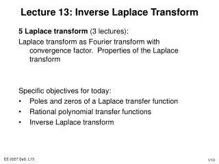
Lecture 13: Inverse Laplace Transform. 5 Laplace transform (3 lectures): Laplace transform as Fourier transform with convergence factor. Properties of the Laplace transform Specific objectives for today: Poles and zeros of a Laplace transfer function Rational polynomial transfer functions

E N D
Lecture 13: Inverse Laplace Transform • 5 Laplace transform (3 lectures): • Laplace transform as Fourier transform with convergence factor. Properties of the Laplace transform • Specific objectives for today: • Poles and zeros of a Laplace transfer function • Rational polynomial transfer functions • Inverse Laplace transform
Lecture 13: Resources • Core material • SaS, O&W, Chapter 9.2(end), 9.3, 9.4 • Recommended material • MIT, Lecture 17, 18
Reminder: Laplace Transforms • Equivalent to the Fourier transform when s=jw • There is an associated region of convergence for s where the (transformed) signal has finite energy. The Laplace transform is only defined for these values • Laplace transform is linear (easy!) • Examples for the Laplace transforms include
Im s-plane – roots of N(s) x x x – roots of D(s) -2 -1 1 Re Ratio of Polynomials • In each of these examples, the Laplace transform is rational, i.e. it is a ratio of polynomials in the complex variable s. • where N and D are the numerator and denominator polynomial respectively. • In fact, X(s) will be rational whenever x(t) is a linear combination of real or complex exponentials. Rational transforms also arise when we consider LTI systems specified in terms of linear, constant coefficient differential equations. • We can mark the roots of N and D in the s-plane along with the ROC • Example 3:
Poles and Zeros • The roots of N(s) are known as the zeros. For these values of s, X(s) is zero. • The roots of D(s) are known as the poles. For these values of s, X(s) is infinite, the Region of Convergence for the Laplace transform cannot contain any poles, because the corresponding integral is infinite • The set of poles and zeros completely characterise X(s) to within a scale factor (+ ROC for Laplace transform) • The graphical representation of X(s) through its poles and zeros in the s-plane is referred to as the pole-zero plot of X(s)
Im x x -1 1 2 Re Example: Poles and Zeros • Consider the signal: • By linearity (& last lecture) we can evaluate the second and third terms • The Laplace transform of the impulse function is: • which is valid for any s. Therefore,
ROC Properties for Laplace Transform • Property 1: The ROC of X(s) consists of strips parallel to the jw-axis in the s-plane • Because the Laplace transform consists of s for which x(t)e-st converges, which only depends on Re{s} = s • Property 2: For rational Laplace transforms, the ROC does not contain any poles • Because X(s) is infinite at a pole, the integral must not converge. • Property 3: if x(t) is finite duration and is absolutely integrable then the ROC is the entire s-plane. • Because x(t) is magnitude bounded, multiplication by any exponential over a finite interval is also bounded. Therefore the Laplace integral converges for any s.
Inverse Laplace Transform • The Laplace transform of a signal x(t) is: • We can invert this relationship using the inverse Fourier transform • Multiplying both sides by est: • Therefore, we can recover x(t) from X(s), where the real component is fixed and we integrate over the imaginary part, noting that ds = jdw
Inverse Laplace Transform Interpretation • Just about all real-valued signals, x(t), can be represented as a weighted, X(s), integral of complex exponentials, est. • The contour of integration is a straight line (in the complex plane) from s-j to s+j (we won’t be explicitly evaluating this, just spotting known transformations) • We can choose any s for this integration line, as long as the integral converges • For the class of rational Laplace transforms, we can express X(s) as partial fractions to determine the inverse Fourier transform.
Im x x -2 -1 Re Example 1: Inverting the Laplace Transform • Consider when • Like the inverse Fourier transform, expand as partial fractions • Pole-zero plots and ROC for combined & individual terms
Im x x -2 -1 Re Example 2 • Consider when • Like the inverse Fourier transform, expand as partial fractions • Pole-zero plots and ROC for combined & individual terms
Lecture 13: Summary • For many signals that are made up of a linear combination of complex exponentials and CT LTI systems that are described by differential equations, the Laplace transform is rational, i.e. it is a ratio of polynomials in s: N(s)/D(s) • The roots of N(s) and D(s) are known as the zeros and poles of the transfer function, respectively. • The Region of Convergence does not contain any poles • The inverse Laplace transform is given by • It is usually calculated by expressing the Laplace transform as partial fractions, and then spotting known relationships (rather than directly evaluating the inverse transform)
Questions • Theory • SaS, O&W, Q9.9, 9.22. Also, prove • Matlab • Verify Q9.9 in Matlab via • >> syms s • >> y = ilaplace(2*(s+2)/(s^2+7*s+12)) • >> t = 0:0.05:2; • >> y1 = subs(y); • >> plot(t,y1); • Do the same for the other examples in the help section for ilaplace. Note that in Matlab dirac(t) is the impulse/delta function d(t) and heaviside(t) is the step function u(t)