Download

1 / 20
200 likes | 393 Views
Lets remember about Goal formulation, Problem formulation and Types of Problem. OBJECTIVE OF TODAY’S LECTURE.

E N D
Lets remember about Goal formulation, Problem formulation and Types of Problem. OBJECTIVE OF TODAY’S LECTURE Today we will discus how to find a solution –is done by a search through the state space. The idea is to maintain and extend a set of partial solution sequences. In this lecture , we show how to generate these sequences and how to keep track of them using suitable data structures. and the process of exploring what the means can do is called search . We show what search can do , how it must be modified to account for adversaries , and what its limitations are.
Generating action sequences To solve the route-finding problem from Arad to Bucharest, for example, we start off with just the initial state, Arad. The first step is to test if this is a goal state. Clearly it is not, but it is important to check so that we can solve trick problems like ‘’ starting in Arad, get to Arad.” Because this is not a goal state, we need to consider some other states. This is done by applying the operators to the current state, thereby generating a new set of states. The process is called expanding the state. In this case, we get three new states,” in Sibiu”, “ In Timisoara,” and “ in Zerind” because there is a direct one-step route from Arad to these three cities. If there were only one possibility, we would just take it and continue. But whenever there are multiple possibilities, we must make a choice about which one to consider further.
Partial search tree for route finding from Arad to Bucharest. Timisora Sibiu Zerind Rimnicu Vilcea Arad Oradea Fagaras Sibiu Bucharest Arad Figure:7.1:- An informal description of the general searchalgorithm.
Data structures for search tress • There are many ways to represent nodes, but in this chapter, we will assume a node is a data structure with five components: • the state in the state space to which the node corresponds; • the node in the search tree that generated this node ( this is called the parent node ); • The operator that was applied to generate the node; • the number of nodes on the path from the root to this node ( the depth of the node); • the path cost of the path form the initial state to the node.
SEARCH STRATEGIES The majority of work in the area of search has gone into finding the right search strategy for problem. In our study of the field we will evaluate strategies in terms of four criteria: Completeness:is the strategy guaranteed to find a solution when there is one? Time complexity:how long does it make to find a solution? Space complexity:how much memory does it need to prefer the search? Optimality: does the strategy find the highest –quality solution when there are several different solutions?
WE KNOW THAT THERE IS TOW CATEGORIES OF SEARCH: UNINFORMED SEARCH INFORMED SEARCH
UNINFORMED SEARCH We will covers six search strategies that come under the heading of uninformed search. The term means that they have no information about the number of steps of the path cost from the current state to the goal- all they can do is distinguish a goal state from a nongoal state. Uniformed search is also sometimes called blind search.
BREADTH-FIRST SEARCH UNIFORM COST SEARCH DEPTH-FIRST SEARCH DEPTH-LIMITED SEARCH ITERATIVE DEEPENING SEARCH BIDIRECTIONAL SEARCH
BREADTH-FIRST SEARCH This is very simple search strategy is a breath-first search. In this strategy, the root node is expanded first, then all the nodes generated by the root node are expanded next, and then their successors, and so on……… function BREADTH-FIRST –SEARCH (problem) returns a solution or failure returns GENERAL-SEARCH (problem, ENQUEUE- AT- END )
Figure:-Time and memory requirements for breadth –first search
18 5 10 12 13 17 56 9 UNIFORM COST SEARCH Uniform cost search modifies the breadth-first strategy by always expanding the lowest-cost node on the fringe (as measured by the path cost g(n)), rather than the lowest-depth node. It is easy to see that breadth-first search is just uniform cost search with g(n) = DEPTH (n). 45 15 50
DEPTH-FIRST SEARCH Depth-first search always expands one of the nodes at the deepest level of the tree. Only when the search hits a dead end
Depth-limited search Depth-limited search avoids the pitfalls of depth-first search by imposing a cutoff on the maximum depth of a path. This cutoff can be implemented with a special depth-limited search algorithm, or by using the general search algorithm with operators that keep track of the depth.
Iterative deepening search Iterative deepening search is a strategy that sidesteps the issue of choosing the best depth limit by trying all possible depth limits: first depth 0, then 2, and so on. The algorithm is shown in below . In effect, iterative deepening combines the benefits of depth-first and breadth-first search. It is optimal ad complete, like breadth-first search, but has only the modest memory requirements of depth-first search. The order of expansions of states is similar to breadth-first, except that some states are expanded multiple times, Figure 7.4 shows the first four iterations of Iterative-Deepening-Search on a binary search tree. function ITERATIVE-DEEPENING-SEARCH (problem) returns a solution sequence inputs: problem, a problem for depth – 0 to do if Depth-Limited-Search (problem, depth) succeeds then return its result end return failure
Figure:7.5 Four iterations of iterative deepening search on a binary tree
(d +1)1 + (d) b + (d- 1)b2 + .... + 3bd-2 + 2bd-1+1bd Again, for b = 10 and d = 5 the number is 6 + 50 + 400 + 3,000 + 20,000 + 100,000 = 123,450
Bi-directional search The idea behind bi-directional search is to simultaneously search both forward from the initial state and backward from the goal, and stop when the two searches meet in the middle (Figure 7.6). For problems where the branches factor is b in both directions, bi-directional search can make a big difference. If we assume as usual that there is a solution of depth d, then the solution will be found in O (2bd/2)= O (b d/2) steps,
Comparing search strategies Figure:7.6:- Evaluation of search strategies. b is the branching factor , d is the depth of solution; m is the maximum depth of the search tree; l is the depth limit.