Download
1 / 31
320 likes | 501 Views
Self Consistent Solar Wind Models. Steven R. Cranmer Harvard-Smithsonian Center for Astrophysics. Self Consistent Solar Wind Models. Outline: Five Necessary “Ingredients” Successes of Wave/Turbulence Models (1D) New Approximations for Wave Reflection (3D).

E N D
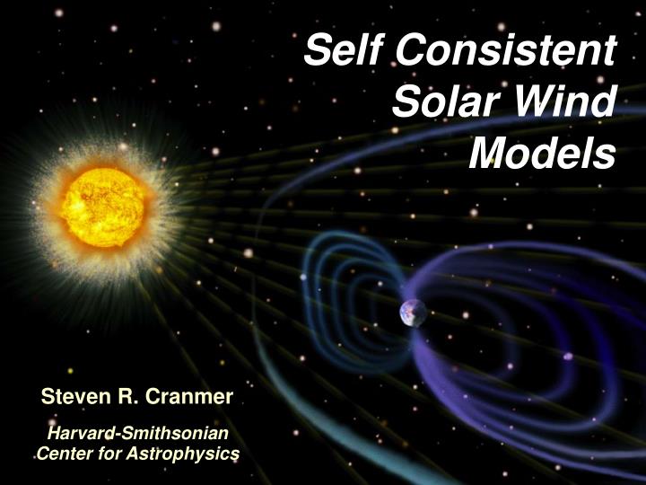
Self ConsistentSolar WindModels Steven R. CranmerHarvard-SmithsonianCenter for Astrophysics
Self ConsistentSolar WindModels • Outline: • Five Necessary “Ingredients” • Successes of Wave/Turbulence Models (1D) • New Approximations for Wave Reflection (3D) Steven R. CranmerHarvard-SmithsonianCenter for Astrophysics
Parker’s isothermal solar wind • Gene Parker (1958) considered the steady-state conservation of mass and momentum in a hot (T ≈ 106 K) corona. • Solutions were independent of the density (everywhere), and they did not require solving the internal energy conservation equation. • In the early 1960s, new models with different T(r) profiles, including those consistent with polytropic (P ~ ργ) equations of state. γ < 1.5 ! • Sturrock & Hartle (1966) included heat conduction (and Tp ≠ Te), and found that energy addition was needed.
Ingredient #1: “real” coronal heating • What determines how much energy is deposited as heat… ultimately from the “pool” of subphotospheric convection? vs. • Waves & turbulent dissipation? • Reconnection / mass input from loops? • How much heating is needed to produce the fast & slow solar wind? ≈8 x 10⁵erg/cm2/s (fast wind) ≈3 x 10⁶erg/cm2/s (slow wind) e.g., Leer et al. (1982)
Ingredient #2: extra momentum sources Contours: wind speed at 1 AU (km/s) • It was realized in the late 1970s that coronal temperatures were probably too low to produce the “fast” solar wind via gas pressure gradients alone. • Just as E/M waves carry momentum and exert pressure on matter, acoustic and MHD waves do work on the gas via similar net stress terms. • To illustrate the effect, I constructed a grid of Parker-like models, with a ~flat Tp(r) and a range of Alfvén wave amplitudes (conserving wave action). P C H
heat conduction radiation losses 5 2 — ρvkT Ingredient #3: self-regulating mass flux • Hammer (1982) & Withbroe (1988) suggested a steady-state energy balance: • Only a fraction of the deposited heat flux conducts down, but in general, we expect that the mass loss rate should be roughly proportional to Fheat. • (In practice, the dependence is ~weaker than linear . . .)
Ingredient #4: in situ conduction & heating • Is the internal energy “game” over by the time the solar wind accelerates to its final terminal speed? • In situ measurements (0.3–5 AU) say no . . . Cranmer et al. (2009) T ~ r–4/3 Proton: 0.3 AU 1 AU 5 AU Electron:
Ingredient #5: funnel-type field expansion • Blah. Πανταρει ! Peter (2001) Fisk (2005) • Empirical models of the open field from the “magnetic carpet” demand superradial expansion in low corona. • UV Doppler blue-shifts are consistent with funnel flows (Byhring et al. 2008; Marsch et al. 2008). • H I Lyα disk intensity in coronal holes isn’t explainable without funnel flows (Esser et al. 2005).
Ingredient #5: funnel-type field expansion • Cranmer & van Ballegooijen (2010) produced Monte Carlo models of the magnetic carpet’s connection to the solar wind. Preliminary models suggest the super-granular network is (at least in part) “emergent” from smaller-scale granule motions , diffusion, & rapid bipole emergence (e.g., Rast 2003; Crouch et al. 2007).
What happens when all of these ingredients are mixed together?
Waves & turbulence in open flux tubes • Photospheric flux tubes are shaken by an observed spectrum of horizontal motions. • Alfvén waves propagate along the field, and partly reflect back down (non-WKB). • Nonlinear couplings allow a (mainly perpendicular) cascade, terminated by damping. (Heinemann & Olbert 1980; Hollweg 1981, 1986; Velli 1993; Matthaeus et al. 1999; Dmitruk et al. 2001, 2002; Cranmer & van Ballegooijen 2003, 2005; Verdini et al. 2005; Oughton et al. 2006; many others)
Dissipation of MHD turbulence • Standard nonlinear terms have a cascade energy flux that gives phenomenologically simple heating: • We used a generalization based on unequal wave fluxes along the field . . . (“cascade efficiency”) Z– Z+ • n = 1: usual “golden rule;” we also tried n = 2. • Caution: this is an order-of-magnitude scaling! (e.g., Pouquet et al. 1976; Dobrowolny et al. 1980; Zhou & Matthaeus 1990; Hossain et al. 1995; Dmitruk et al. 2002; Oughton et al. 2006) Z–
Self-consistent 1D models • Cranmer, van Ballegooijen, & Edgar (2007) computed solutions for the waves & background one-fluid plasma state along various flux tubes... going from the photosphere to the heliosphere. • The only free parameters: radial magnetic field & photospheric wave properties. • Some details about the ingredients: • Alfvén waves: non-WKB reflection with full spectrum, turbulent damping, wave-pressure acceleration • Acoustic waves: shock steepening, TdS & conductive damping, full spectrum, wave-pressure acceleration • Radiative losses: transition from optically thick (LTE) to optically thin (CHIANTI + PANDORA) • Heat conduction: transition from collisional (electron & neutral H) to a collisionless “streaming” approximation
Magnetic flux tubes & expansion factors A(r) ~ B(r)–1 ~ r2 f(r) (Banaszkiewicz et al. 1998) Wang & Sheeley (1990) defined the expansion factor between “coronal base” and the source-surface radius ~2.5 Rs. TR polar coronal holes f ≈ 4 quiescent equ. streamers f ≈ 9 “active regions” f ≈ 25
Results: turbulent heating & acceleration T (K) Ulysses SWOOPS Goldstein et al. (1996) reflection coefficient
Summary of other results • Wind speed is anti-correlated with flux-tube expansion & height of critical point. • Temperature (Matthaeus, Elliott, & McComas 2006) • Frozen-in charge states [O7+/O6+] • The FIP effect [Fe/O] • Specific entropy [ln(T/nγ–1)] (Pagel et al. 2004) • Turbulent fluctuation energy (Tu et al. 1992) • Models match in situ data that correlate wind speed with: (Zurbuchen et al. 1999) • Integrated heat fluxes |Fheat| match empirical req’s: 106 to 3x10⁶ erg/cm2/s. • Comparison with remote-sensing data (e.g., UVCS) isn’t as far along, because the models are one-fluid… the data showcase multi-fluid collisionless effects. • The turbulent heating rate in the corona scales directly with the mean magnetic flux density there, as is inferred from X-rays (e.g., Pevtsov et al. 2003). For more information, see Cranmer (2009, Living Reviews in Solar Phys.,6, 3)
TZ Challenge #2: is slow wind composition open/closed? • FIP effect modeled with Laming (2004) theory: Alfven waves exert “pressure” on ions, but not on neutrals in upper chromo. Ulysses SWICS • Wave pressure is automatically calculated in the model. • In chromosphere, | awp / g | ≈ 0.1, but it acts over ~tens of scale heights. • Note that in these models, the “hole/streamer boundary slow wind” has fast-wind-like abundances. Only the “active region slow wind” has enhanced low-FIP abundances. Cranmer et al. (2007)
TZ Challenge #3: how does heating affect slow/fast wind? • How do fast-wind properties in interplanetary space vary from the 1996–1997 minimum to the present minimum? Fractions given as “(new–old)/old” • “New” magnetic field model was run with same parameters as old model. Ulysses polar data WTD model output speed density Temp. Pgas Pdyn –03 % –17 % –14 % –28 % –22 % +01 % –22 % –08% –21 % –27 % v,n,T (output) B field (input) (McComas et al. 2008) (Cranmer et al. 2010, SOHO-23 Proc.)
What’s stopping us from including this in 3D “global MHD” models of the Sun-heliosphere system? → Non-WKB Alfvén wave reflection!
How is wave reflection treated? • At photosphere:empirically-determined frequency spectrum of incompressible transverse motions (from statistics of tracking G-band bright points) • At all larger heights:self-consistent distribution of outward (z–) and inward (z+) Alfvenic wave power, determined by linear non-WKB transport equation: 3e–5 1e –4 3e –4 0.001 0.003 0.01 0.03 0.1 0.3 0.9 “refl. coef” = |z+|/|z–| TR
Reflection in simple limiting cases . . . • Many earlier studies solved these equations numerically (e.g., Heinemann & Olbert 1980; Velli et al. 1989, 1991; Barkhudarov 1991; Cranmer & van Ballegooijen 2005). • As wave frequency ω→ 0, the superposition of inward & outward waves looks like a standing wave pattern: phase shift → 0 • As wave frequency ω→∞, reflection becomes weak . . . phase shift → – π/2 • Cranmer (2010) presented approximate “bridging” relations between these limits to estimate the non-WKB reflection without the need to integrate along flux tubes. • See also Chandran & Hollweg (2009); Verdini et al. (2010) for other approaches!
Results: numerical integration vs. approx. 3e–5 1e –4 3e –4 0.001 0.003 0.01 0.03 0.1 0.3 0.9 “refl. coef” = |z+|/|z–| TR 3e–5 1e –4 3e –4 0.001 0.003 0.01 0.03 0.1 0.3 0.9 ω0
Results: coronal heating rates • Each “row” of the contour plot contributes differently to the total, depending on the power spectrum of Alfven waves . . . Tomczyk & McIntosh (2009) f –5/3 Cranmer & van Ballegooijen (2005) observational constraints on heating rates
Conclusions • It is becoming easier to include “real physics” in 1D → 2D → 3D models of the Sun-heliosphere system. • Theoretical advances in MHD turbulence continue to help improve our understanding about coronal heating and solar wind acceleration. • We still do not have complete enough observational constraints to be able to choose between competing theories. vs. For more information: http://www.cfa.harvard.edu/~scranmer/
Multi-fluid collisionless effects! O+5 O+6 protons electrons coronal holes / fast wind (effects also present in slow wind)
Intensity modulations . . . • Motion tracking in images . . . • Doppler shifts . . . • Doppler broadening . . . • Radio sounding . . . Low-freq. waves: remote-sensing techniques The following techniques are direct… (UVCS ion heating is more indirect) Tomczyk et al. (2007)
Wave / Turbulence-Driven models • Cranmer & van Ballegooijen (2005) solved the transport equations for a grid of “monochromatic” periods (3 sec to 3 days), then renormalized using photospheric power spectrum. • One free parameter: base “jump amplitude” (0 to 5 km/s allowed; ~3 km/s is best)
Results: in situ turbulence • To compare modeled wave amplitudes with in-situ fluctuations, knowledge about the spectrum is needed . . . • “e+”: (in km2 s–2 Hz–1 ) defined as the Z– energy density at 0.4 AU, between 10–4 and 2 x 10⁻⁴ Hz, using measured spectra to compute fraction in this band. Helios (0.3–0.5 AU) Tu et al. (1992) Cranmer et al. (2007)
New result: solar wind “entropy” • Pagel et al. (2004) found ln(T/nγ–1) (at 1 AU) to be strongly correlated with both wind speed and the O7+/O6+ charge state ratio. (empirical γ = 1.5) • The Cranmer et al. (2007) models (black points) do a reasonably good job of reproducing ACE/SWEPAM entropy data (blue). • Because entropy should be conserved in the absence of significant heating, the quantity measured at 1 AU may be a long-distance “proxy” for the near-Sun locations of strong coronal heating.
B ≈ 1500 G (universal?) f ≈ 0.002–0.1 B ≈ f B , . . . . . . • Thus, . . . and since Q/Q ≈ B/B , the turbulent heating in the low corona scales directly with the mean magnetic flux density there (e.g., Pevtsov et al. 2003; Schwadron et al. 2006; Kojima et al. 2007; Schwadron & McComas 2008). New result: scaling with magnetic flux density • Mean field strength in low corona: • If the regions below the merging height can be treated with approximations from “thin flux tube theory,” then: B ~ ρ1/2 Z± ~ ρ–1/4 L┴ ~ B–1/2