Download

1 / 62
760 likes | 2.12k Views
Chapter 9 Phase Diagrams–Equilibrium Microstructural Development. This chapter, 9, deals with the following topics; 9.1 The Phase Rule 9.2 The Phase Diagram 9.3 The Lever Rule 9.4 Microstructural Development During Slow Cooling.

E N D
Chapter9Phase Diagrams–Equilibrium Microstructural Development
This chapter, 9, deals with the following topics; 9.1 The Phase Rule 9.2 The Phase Diagram 9.3 The Lever Rule 9.4 Microstructural Development During Slow Cooling
It is well known that the properties of materials depend on the their atomic and microscopic structures. To understand the nature of the microstructure-sensitive properties of eng- ineering materials, one has to explore the way in which microstructure is developed. An important tool in this exploration is the phase diagram, which is a map that will guide us in answering the general questions; 1). What microstructure should exist at a given temperature for a given material composition? (The answer is given by equilibrium nature) 2). How fast will the microstructure form at a given temperature? And What temperature versus time history will result in an optimal microstructure? (The answers for these questions are in Ch. 10)
Dependency of yield strength and microstructure of Fe-0.8%C steel upon cooling rate from 900 degree C holding
9.1 The Phase Rule Phase Rule: The rule which identifies the number of microscopic phases associated with a given state condition, a set of values for temperature, pressures, and other variables that describe the nature of the material. A phaseis a chemically and structurally homogeneous portion of the micro- structure. A single-phase microstructure can be polycrystalline (Fig. 9.1), but each crystal grain differs only in crystalline orientation, not in chemical composition. A component is a distinct chemical substance from which the phase is formed, in other words, one or more components may make a phase. Ex; ①. in Ch 4, it is shown that Cu-Ni (two components) form a complete single solid solution phase. ②. The two components ofMgO and NiO form another solid solution in a way similar to that Cu and Ni . In case of two components system, if the solute is added over the solid solubility limit, then two phases are formed.
A single phase of one component, Mo. Figure 9.1Single-phase microstructure of commercially pure molybdenum, 200×. Although there are many grains in this microstructure, each grain has the same uniform composition.
Two-phase (αiron and carbide) microstructure made of two components of Fe and C. This two phase mixture structure is called “ pearlite”. Figure 9.2Two-phase microstructure of pearlite found in a steel with 0.8 wt % C, 650 ×. This carbon content is an average of the carbon content in each of the alternating layers of ferrite (with <0.02 wt % C) and cementite (a compound, Fe3C, which contains 6.7 wt % C). The narrower layers are the cementite phase. (From ASM Handbook, Vol. 9: Metallography and Microstructures, ASM International, Materials Park, OH, 2004.) Explain the property of this pearlite structure.
The degrees of freedom are the number of independent variables available to the system. Introduction of Gibbs Phase rule : F=C-P+2 where F is the number of degrees of freedom, C is the number of components, and P is the number of phases, and 2 indicates two state variables of temper-ature and pressure. For most solid materials, the effect of pressure is so slight that pressure is fixed to be 1 atm. In this case the Phase Rule becomes; F=C-P+1 A pure metal, at precisely its melting point, has no degrees of freedom. In other words, at this condition, or state, the metal exists in two phases in equilibrium, i.e., solid and liquid phases simultaneously. Applying the phase rule at Mpt.; C=1, P=2, → F=1-2+1=0. This F=0 means both temperature and composition can not be changed. Slightly above Mpt ; all liquid (one phase), below Mpt ; all solid one phase). In these cases of at T>Mpt and T<Mpt, ; C=1, P=1→ F=1-1+1=1 This F=1 means even though, one state variable, T, varies, the phase is not changed, i.e., liquid or solid phase does not change with temperature.
B • Figure 9.3(a) Schematic representation of the one-component phase diagram for H2O. (b) A projection of the phase diagram information at 1 atm generates a temperature scale labeled with the familiar transformation temperatures for H2O (melting at 0°C and boiling at 100°C). A • (fixed) One Phase Case : At point “A”, T=Mpt, and P=2 (solid and liquid) → C=1, P=2, → F=1-2+1=0. At point “B”, T=Bpt, and P=2 (gas and liquid) → C=1, P=2, → F=1-2+1=0. But, in between A and B, C=1, P=1, → F=1-1+1=1, This 1 indicates that “temperature can be changed freely from 0 to 100oC, keeping one phase of liquid. (Consider, what happens if pressure is not fixed.)
Figure 9.4(a) Schematic representation of the one-component phase diagram for pure iron. (b) A projection of the phase diagram information at 1 atm generates a temperature scale labeled with important transformation temperatures for iron. This projection will become one end of important binary diagrams, such as that shown in Figure 9.19 The situations are same as those of the previous Fig. 9.4 (H2O). In this solid case, practically pressure does not affect the phase rule.
Examples and Practice Problems : Students are asked to review the “Example” of 9.1 and solve the “Practice Problem” of 9.1 in the text.
9.2 The Phase Diagram A phase diagram is any graphical representation of the state variables asso-ciated with microstructures through Gibbs phase rule. In other words, phase diagram is considered as the maps of the phases with temperature. Depend on the number on components composing a material, the phase diagram becomes different. Two-component systems are called Binary Diagram. (C=2 in the Gibbs phase rule) Three-component systems are called Ternary Diagram. (C=3 in the Gibbs phase rule) For four-component of more component systems can not be drawn. In this text book, only binary diagrams will be explained.
Examples of this type of diagram; Cu-Ni in metal system and MgO-NiO in ceramics system. Figure 9.5Binary phase diagram showing complete solid solution. The liquid-phase field is labeled L, and the solid solution is designated SS. Note the two-phase region labeled L + SS. Explain the meaning of the diagram and notations such as A, B, L and SS, liquidus, solidus ect. A and B are completely soluble each other both in L & S phases The simplest type of phase diagram in binary system in which the two component exhibit complete solid solution.
of B in L phase Explain the meaning of “tie line”: BL Figure 9.6The compositions of the phases in a two-phase region of the phase diagram are determined by a tie line (the horizontal line connecting the phase compositions at the system temperature). BSS of B in SS phase
(Gibbs Phase Rule) (T & C) Liquid solution field Melting point of B, “invariant point”. Figure 9.7Application of Gibbs phase rule (Equation 9.2) to various points in the phase diagram of Figure 9.5. L+SS region Explain the application of Gibbs phase rule. The physical meaning also. F=0 (T & C) Solid solution field
Boundary between L1 and SS1. Figure 9.8Various microstructures characteristic of different regions in the complete solid-solution phase diagram. SS1 L1 Grain boundary between SS grains. SS Explain the process of solidification.
Hume-Rothery rule; Figure 9.9Cu–Ni phase diagram.
Construction of the Co-Ni equilibrium phase diagram from liquid-solid cooling curves (a) Cooling curves. (b) equilibrium phase diagram
Hume-Rothery rule for metal is still applicable for oxide system. In this case, the relative size of cations has to be similar in size. Figure 9.10NiO–MgO phase diagram. Check ionic size of Ni and Mg. (Not in wt%)
A and B are completely insoluble each other. This is an opposite case of the complete SS system. Hypo eutectic Hyper eutectic Figure 9.11Binary eutectic phase diagram showing no solid solution. This general appearance can be contrasted to the opposite case of complete solid solution illustrated in Figure 9.5. LEC Eutectic reaction : LEC→A+B cooling below eutectic T.
L Leut Figure 9.12Various microstructures characteristic of different regions in a binary eutectic phase diagram with no solid solution. Lhyper Lhypo L2 A B L1 L2 L1 B A Teut The remaining L1 becomes Leut at Teut and solidifies eutectic microstructure below Teut. Similar microstructure is obtained for hyper case. (Why?) B A Since randomly mixed liquid of A & B are solidifies into two separate solid phases of A & B at one temperature, the resulting microstructure must be fine. Depend on system, it will be lamellar or nodular structure of fine.
This real phase diagram for Al-Si system is the close approximation to Fig. 9.11 in that aluminum dissolves some Si to make several useful Al alloys. Figure 9.13Al–Si phase diagram. In Si side, extremely small amount of aluminum can be dissolved in silicon. To make p-type semiconductors, Al is doped in Si. Since the solid solubi-lity of Al in Si is too small, there will be a limit of Al doping amount in Si. (See Ch. 13)
The two components of A and B are partially soluble in each other to form α & β solid solution phases of A & B. Teut Leutα + β. Figure 9.14Binary eutectic phase diagram with limited solid solution. The only difference between this diagram and the one shown in Figure 9.11 is the presence of solid-solution regions α and β. Usually, α & β have different crystal structures and properties. Because these two components are different chemically & physically. Leut
L L1 Figure 9.15Various microstructures characteristic of different regions in the binary eutectic phase diagram with limited solid solution. This illustration is essentially equivalent to the illustration shown in Figure 9.12, except that the solid phases are now solid solutions (α and β) rather than pure components (A and B). α3 L2 β1 α β α1 α1, α2 & α3 are all the same phase but differ-ent B content. Explain the phase transformation procedures for “hypo” & “hyper” compositions also.
Figure 9.16Pb–Sn phase diagram. (includes common solder alloys) α + L ④ ③ ② ① (Allotropic transformation temp.) 5 Low melting range of this system allows for joining of metals by convenient heating methods. ①. For sealing containers and coating & joining metals used above 120oC. ②. For sealing cellular automobile radiators & filling seams & dents in automobile bodies. ③. For general-purpose solders. These solders have a characteristic past like consistency during soldering, associated with the two-phase liquid plus solid region just above the eutectic temperature. ④. For heat sensitive electronic parts that require minimum heating.
Figure 9.17This eutectoid phase diagram contains both a eutectic reaction (Equation 9.3) and its solid-state analog, a eutectoid reaction (Equation 9.4). Eutectoid phase transformation is; Solid 1→Solid 2 + Solid 3. (γ→α+β) This reaction takes place in solid phase, means reaction is very slow ∵Solid state diffusion is involved. So grain structure is very fine to have high strength. More detailed studies will be given later for steel making!
Figure 9.18Representative microstructures for the eutectoid diagram of Figure 9.17. γ 1 ∵High temp reaction α + β
Schematic illustration of various eutectic structures(a) lamellar, (b) rodlike,(c) globular, (d) acicular
This is most important commercial phase diagram and it provides the major scientific basis for the iron and steel industries. This diagram is representative of the microstructural development in many related systems with three or more components, e.g., stainless steels that include large amount of Cr. Figure 9.19Fe–Fe3C phase diagram. Note that the composition axis is given in weight percent carbon even though Fe3C, and not carbon, is a component. In stead of carbon, Fe3C is a compon-ent in this system, the composition axis is customarily given in wt% C. This Fe-Fe3C diagram is not a true equilibrium diagram.∵The most stable form of C is graphite, but the rate of graphitization is too slower than Fe3C, the meta stable Fe3C is considered as one of the components of this system. Fe3C
Thermodynamically and fundamentally, this Fe-C diagram is the real equilibr-ium diagram under the condition of extremely slow cooling. Figure 9.20Fe–C phase diagram. The left side of this diagram is nearly identical to the left side of the Fe–Fe3C diagram (Figure 9.19). In this case, however, the intermediate compound Fe3C does not exist. Practical method to promote graphite precipitation is adding small amount of third component, such as Si. Typically 2~3% Si addition stabilizes graphite precipitation.
So far it is known that the pure compo-nents have had distinct melting point. However, in some systems, the compo-nents will form stable compounds that may not have such a distinct Mpt. Incongruent melting : Temperature Composition of liquid in B formed upon melting of AB is B’, not 50%B. Figure 9.21Peritectic phase diagram showing a peritectic reaction (Equation 9.5). For simplicity, no solid solution is shown. In Fig. 9.21, an example shows that A and B form the stable compound, AB, which does not melt at a single tempera-ture as do components A and B. Incongruent melting of AB Congruent Melting : A liquid formed upon melting has the same composition as the melted solid. The compound, AB, is said to undergo Incongruent melting, because the liquid formed upon melting has a composition other than AB. (See the figure, 50A - 50B) ; i.e., AB B + L(composition is not AB) This is called Peritectic Reaction. B’ melting
This peritectic reaction is not common for metal alloy system. L B L1 Figure 9.22Representative microstructures for the peritectic diagram of Figure 9.21. L+B 1 AB Intermediate compound, or intermediate phase, AB : A chemical compound formed between two components of A and B in a binary system.
This binary diagram is as important to the ceramic industry as the Fe-Fe3C diagram is to the steel industry. Silica brick is used above 1,600oC, it is important to keep the Al2O3 content as low as possible to minimize the liquid phase. A small amount of liquid is tolerable. The composition of Al2O3 (impurity) in refractory silica brick (SiO2 ) is 0.1~0.6 mol%. Figure 9.23Al2O3–SiO2phase diagram. Mullite is an intermediate compound with ideal stoichiometry 3Al2O3 · 2SiO2. Peritectic reaction A dramatic increase in refractoriness, or temperature resistance, occurs at the compo-sition of the incongrue-ntly melting compound, Mullite (3Al2O3•2SiO2). The Max. Temp. to be safely used is 1,890oC. In mullite, Al2O3 has to be higher than 60 mol% not to have liquid phase at the elevated temp. Safe comp. of Al2O3 in mullite for high temp. safe use with out liquid phase. Composion for common fireclay refractories, therefore, the use temp. has to be below 1,587oC Comp. range for high-alumina refractories.
congruently melting point The phase AB in the figure is the intermediate compound which is relatively common occurrence in binary system. In this figure, the intermediate compound is not involved in the peritectic reaction. But this phase has the congruent melting point. Figure 9.24(a) Binary phase diagram with a congruently melting intermediate compound, AB. This diagram is equivalent to two simple binary eutectic diagrams (the A–AB and AB–B systems). (b) For analysis of microstructure for an overall composition in the AB–B system, only that binary eutectic diagram need be considered. An interesting point in this system is that it is equivalent to two adjacent binary eutectic diagrams of the type without any terminal solid solubility. If we want study AB-B binary system, one may think A-AB is not existing, so consider only AB-B part of the diagram counting the overall composition (counting 100 % scale) between AB and B.
Figure 9.25 (a) A relatively complex binary phase diagram. (b) For an overall composition between AB2 and AB4, only that binary eutectic diagram is needed to analyze microstructure. A binary system with an overall composition between AB2 and AB4 is considered only.
The intermediate compound of spinel has the component of stoichiometry MgO · Al2O3. Since the congruent melting point of this spinel is almost 2,100oC, these refractories are widely used in industry. Figure 9.26MgO–Al2O3 phase diagram. Spinel is an intermediate compound with ideal stoichiometry MgO · Al2O3or MgAl2O4. (An important family of mag-netic materials is based on the chemistry and crystal structure of spinel. This will be studied in Ch. 13.) MgAl2O4
This Al-Cu system is a good example of general diagram having many intermediate compounds. Figure 9.27Al–Cu phase diagram. Composition range of very useful Al-Cu alloys Less than 5%Cu alloys are very important age hardenable alloys used for aerospace materials. The detailed contents ofaging heat treatment will be discussed in Ch. 10.4.
This Cu-Zn system is another example of complex diagram which is used for the design and production procedures for “brass” in Cu rich region. For example, many commercial brass compositions lie in the single-phase of α region shown with red line. Useful range for brass Figure 9.28Cu–Zn phase diagram.
This CaO–ZrO2phase diagram is an example of a general diagram of a ceramic system. Heating, +ᅀV ZrO2 : Monoclinic tetragonal. This increased ᅀVdue to phase transfor-mation creates structural catastrophic failure to the brittle ceramic. By adding ~20 mol% CaO, as it is seen in the diagram, one phase of solid solution is formed and so there is no danger of failure from RT up to ~2,500oC. This is called “stabilized zirconia” and is safely used high temperature refractory, structural material. at 1,000oC Figure 9.29CaO–ZrO2phase diagram. The dashed lines represent tentative results. ZrO2-Y2O3 system also gives similar effect as do CaO–ZrO2.
Examples and Practice Problems : Students are asked to review the “Example” of 9.2 and solve the “Practice Problem” of 9.2 in the text.
9.3 The Lever Rule In Sec. 9.2, we studied the use of phase diagram to determine the phase present at equilibrium in a given system and their corresponding microstructure. In Fig. 9.6, the “tie line” has been introduced to give the composition of each phase in the two-phase region. We now extend this analysis to determine the amount of each phase in the two-phase region using the “tie line”. The relative amounts of the two phases in the microstructure are easily calculated from a mass balance.
Mass-balance calculation : A 50g + B50g =Tot100g 1). Assume the total mass is 100g. Therefore, mL + mSS =100g = mtotal(overall mass balance) (9.6) Tie line Figure 9.30A more quantitative treatment of the tie line introduced in Figure 9.6 allows the amount of each phase(L and SS) to be calculated by means of a mass balance (Equations 9.6 and 9.7). %B in L 2). The amount of B in L is 30% and B in SS is 80%. And the amount of B in the overall system is defined to be 50%. Therefore, Btotal in alloy is; 0.3mL + 0.8mSS = 0.5(100g) = 50g (9.7) mL mSS %B in SS 3). Two equations of (9.6) & (9.7) and two unknowns of mL & mSS, ∴one can get the values of mL=60g & mSS =40g.
• • At T1, β just begins to be precipitated from α T1 • • x xα As T decreases from T1 to T2, T2 xβ The amount of β increased up to mβ, and α decreased down to mα. Figure 9.31The lever rule is a mechanical analogy to the mass-balance calculation. The (a) tie line in the two-phase region is analogous to (b) a lever balanced on a fulcrum. mα mβ For two phases, α andβ, the general mass balance will be xαmα+ xβmβ= x(mα+mβ)(9.8) Eqn. (9.8) can be rearranged to give the relative amount of each phase in terms of compositions; (b) mα Xβ- x X - xα mβ (9.9) and (9.10) = = mα+mβ mα+mβ Xβ- xα Xβ- xα These two eqns. Constitute the lever rule. Its utility is due to the fact that it can be visu-alized so easily in terms of the phase diagram.
Examples and Practice Problems : Students are asked to review the “Example” of 9.3 ~9.5 and solve the “Practice Problem” of 9.3 ~9.5 in the text.
9.4 Microstructural Development During Slow Cooling So far we have studied to decide phase compositions and to calculate the amounts of the phases using the binary phase diagram. Now we are going to study how the microstructures are formed in metals. Microstructure is developed in the process of solidification. To begin with, we consider only the case of slow cooling, that is chemical equilibrium is essentially maintained at all points along the cooling path. (In the section of heat treatment, in Ch. 10, the time-dependent microstructure changes is discussed.)
Microstru-cture Amount of SS trnasformed Figure 9.32Microstructural development during the slow cooling of a 50% A–50% B composition in a phase diagram with complete solid solution. At each temperature, the amounts of the phases in the microstructure correspond to a lever-rule calculation. The microstructure at T2 corresponds to the calculation in Figure 9.30. 50 of B, %
Eutetic reaction : Leut → α + β Teut The relative amounts of αand βjust below Teut are same as shown in the diagram. Figure 9.33Microstructural development and phase calculation during the slow cooling of an eutectic composition. β α xα xβ xeut Xα: %B in αphase. xβ : %B in β phase. xeut : %B in Leutphase. Using these composition data, the following relative amount of α and β are calculated. , (% B) β Xβ - xeut Anti lever rule β = α= Xβ - xα
1). At T = Teut +1 : Primary alpha, αp , formed. Wtofαp= Eutetic reaction : Leut → α + β Teut 55 - 40 X 100= 60 55 - 30 100 g Therefore, wt of αp = 60 g. Therefore, wt of Leut = 40 g. Calculation of the transformed phase amount during the slow cooling of a hypo-eutectic composition. αp α Leut Teut +1 xα xβ αe xeut βe 2). At T = Teut -1 : The remaining liquid, Leut with composition of 55% B=xeut, hastheeutectic reaction to form αeand βe. 55 90 30 40 , (% B) Teut -1 90 - 55 Leut(40g) αe+ βe; Wt of αe = X 40 =23.3 g β 90 - 30 Therefore, one can get the wt of βe as (40-23.3=)16.7g ∴Total wt α = 60 + 23.3=83.3g, Total wt β = 16.7g. β =
Calculation of the transformed phase amount during the slow cooling of a hyper-eutectic composition. The main idea of calculation is similar to that for the hypo-eutectic composition. The only difference is, before the eutectic reaction, primary β is formed and then the remaining liquid phase is experiencing eutectic reaction at below the eutectic temperature. Usually, α phase is soft and β phase is hard and brittle. Therefore, depend on which phase is continuous, the mechanical property of the alloy changes very significantly. 기계적성질 설명 추가.