Download
1 / 57
650 likes | 999 Views
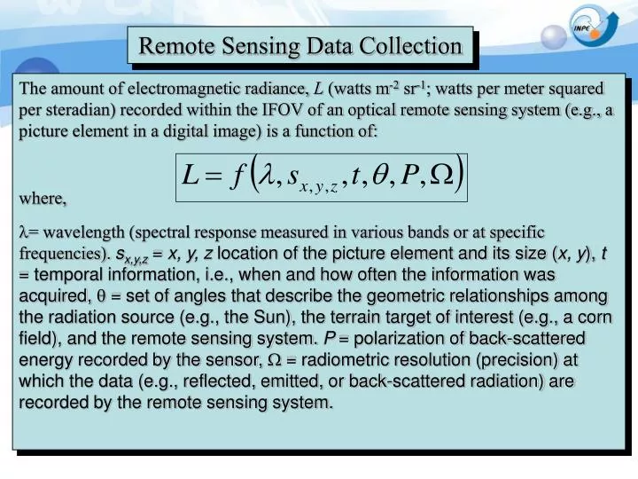
Remote Sensing Data Collection. The amount of electromagnetic radiance, L (watts m -2 sr -1 ; watts per meter squared per steradian) recorded within the IFOV of an optical remote sensing system (e.g., a picture element in a digital image) is a function of: where,

E N D
Remote Sensing Data Collection • The amount of electromagnetic radiance, L (watts m-2 sr-1; watts per meter squared per steradian) recorded within the IFOV of an optical remote sensing system (e.g., a picture element in a digital image) is a function of: • where, • = wavelength (spectral response measured in various bands or at specific frequencies). sx,y,z= x, y, z location of the picture element and its size (x, y), t = temporal information, i.e., when and how often the information was acquired, q = set of angles that describe the geometric relationships among the radiation source (e.g., the Sun), the terrain target of interest (e.g., a corn field), and the remote sensing system. P= polarization of back-scattered energy recorded by the sensor, W = radiometric resolution (precision) at which the data (e.g., reflected, emitted, or back-scattered radiation) are recorded by the remote sensing system.
Remote Sensing Data Collection sx,y,z= x, y, z location of the picture element and its size (x, y) t = temporal information, i.e., when and how often the information was acquired q = set of angles that describe the geometric relationships among the radiation source (e.g., the Sun), the terrain target of interest (e.g., a corn field), and the remote sensing system P= polarization of back-scattered energy recorded by the sensor W = radiometric resolution (precision) at which the data (e.g., reflected, emitted, or back-scattered radiation) are recorded by the remote sensing system.
Platforms • Geostationary Altitudes aprox. 36,000 kilometers Satellites at very high altitudes in which view the same portion of the Earth's surface at all times have geostationary orbits. They have speeds which match the rotation of the Earth so they seem stationary, relative to the Earth's surface. This allows the satellites to observe and collect information continuously over specific areas.
Platforms • Polar Orbit Altitudes aprox. 800 kilometres Follow an orbit (basically north-south) which, in conjunction with the Earth's rotation (west-east), allows them to cover most of the Earth's surface over a certain period of time. Many of these satellite orbits are also sun-synchronous such that they cover each area of the world at a constant local time of day called local sun time. At any given latitude, the position of the sun in the sky as the satellite passes overhead will be the same within the same season.
Satellite Swath • The area of the earth which is imaged during a satellite orbit is referred to as the satellite swath and can range in width from ten to hundreds of kilometers. http://hosting.soonet.ca/eliris/remotesensing/bl130lec11.html
Instantaneous Field of View (IFOV) • The IFOV is the angular cone of visibility of the sensor (A) and determines the area on the Earth's surface which is "seen" from a given altitude at one particular moment in time (B). • The size of the area viewed is determined by multiplying the IFOV by the distance from the ground to the sensor (C). This area on the ground is called the resolution cell and determines a sensor's maximum spatial resolution
DIGITAL IMAGE A photograph could also be represented and displayed in a digital format by subdividing the image into small equal-sized and shaped areas, called picture elements or pixels, and representing the brightness of each area with a numeric value or digital number.
Digital Image Digital Number 0 128 255
Remote Sensor Resolution 10 m • Spatial - the size of the field-of-view, e.g. 10 x 10 m. • Spectral - the number and size of spectral regions the sensor records data in, e.g. blue, green, red, near-infrared thermal infrared, microwave (radar). • Temporal - how often the sensor acquires data, e.g. every 30 days. • Radiometric - the sensitivity of detectors to small differences in electromagnetic energy. 10 m B G R NIR Jan 15 Feb 15 Jensen, 2007
Radiometric Resolution Imagery data are represented by positive digital numbers which vary from 0 to (one less than) a selected power of 2. Each bit records an exponent of power 2 = n bit = 2n The maximum number of brightness levels available depends on the number of bits used in representing the energy recorded. 1 bit (2 gray tone) 5 bit (32 gray tone) The radiometric resolution of an imaging system describes its ability to discriminate very slight differences in energy. .
Radiometric Resolution By comparing a 2-bit image with an 8-bit image, we can see that there is a large difference in the level of detail discernible depending on their radiometric resolutions. Resolução = 2 bits = 22 = 4 níveis de cinza Resolução = 8 bits = 28 = 256 níveis de cinza
RadiometricResolution 7-bit (0 - 127) 0 8-bit (0 - 255) 0 9-bit (0 - 511) 0 10-bit (0 - 1023) 0 Jensen, 2007
Spatial Resolution The detail discernible in an image is dependent on the spatial resolution of the sensor and refers to the size of the smallest possible feature that can be detected.
Spatial Resolution Imagery of residential housing in Mechanicsville, New York, obtained on June 1, 1998, at a nominal spatial resolution of 0.3 x 0.3 m (approximately 1 x 1 ft.) using a digital camera. Jensen, 2007
Spatial resolution Sensors
Spectral Resolution Spectral resolution describes the ability of a sensor to define fine wavelength intervals. The finer the spectral resolution, the narrower the wavelength range for a particular channel or band.
Bands • Satellite sensors measure energy from particular set of wavelengths dl, which are referred to as “bands” and numbered in increasing order from shortwave to longwave. Band dl (mm) Band 1 Band 2 Band 3 Band 4 Band 5 Band 6 Band 7
TemporalResolution Remote Sensor Data Acquisition June 1, 2006 June 17, 2006 July 3, 2006 16 days Jensen, 2007
Remote Sensing Process • From Beginning to End Seven elements of the RS process A Energy Source or Illumination B Radiation and the Atmosphere C Interaction with the Target D Recording of Energy by the Sensor E Transmission, Reception, and Processing F Interpretation and Analysis G Application
Key Concepts in Remote Sensing • Digital Image Processing Techniques • a. Preprocessing Radiometric Correction Geometric Rectification • b. Image Enhancements • c. Spectral Transformations • d. Atmospheric Corrections • e. Image Classification Techniques
Pre-processing it can impact subsequent Error occurs during data acquisition process data analysis Necessary to correct the data Pre-processing • Sources errors: • Internal errors – created by instrument itself • External errors – created by platform, atmosphere, scene characteristics (variable)
Pre-processing • Aim to corrected image close as possible: radiometrically & geometrically – to radiant energy characteristics of original scene • Pre-processing operations, sometimes referred to as image restoration and rectification it can impact subsequent Error occurs during data acquisition process data analysis Necessary to correct the data Pre-processing
Radiometric correction • Radiometric correction is the operation to intend to remove systematic or random noise affecting the amplitude (brightness) of an image. • Radiometric problems can be introduced during: • imaging , • digitalization, • transmission. • Goal to restore an image to the condition it would have been if the imaging process were perfect. • Example Radiometric problems • striping • (partially) missing lines • sensor calibration
Radiometric Problems • Exemples noaa15 • Line dropout • Striping or banding
Radiometric correction Radiometric correction is used to modify DN values to account for noise, i.e. contributions to the DN that are a result of… a. the intervening atmosphere b. the sun-sensor geometry c. the sensor itself We may need to correct for the following reasons: a. Variations within an image (speckle or striping)b. between adjacent or overlapping images (for mosaicing)c. between bands (for some multispectral techniques)d. between image dates (temporal data) and sensors
Geometric Distortion geometric distortion due to: • the perspective of the sensor optics, • the motion of the scanning system, • the motion and (in)stability of the platform, • the platform altitude and velocity, • the terrain relief, and • the curvature and rotation of the Earth.
Geometric correction • Account for distortion in image due to motion of platform and scanner mechanism • Particular problem for airborne data: distortion due to roll, pitch, yaw From:http://liftoff.msfc.nasa.gov/academy/rocket_sci/shuttle/attitude/pyr.html
Geometric correction • Airborne data over Barton Bendish, Norfolk, 1997 • Resample using ground control points • various warping and resampling methods • nearest neighbour, bilinear or bicubic interpolation.... • Resample to new grid (map)
Resampling methods New DN values are assigned in 3 ways a.Nearest Neighbour Pixel in new grid gets the value of closest pixel from old grid – retains original DNs b. Bilinear Interpolation New pixel gets a value from the weighted average of 4 (2 x 2) nearest pixels; smoother but ‘synthetic’ c. Cubic Convolution (smoothest) New pixel DNs are computed from weighting 16 (4 x 4) surrounding DNs http://www.geo-informatie.nl/courses/grs20306/course/Schedule/Geometric-correction-RS-new.pdf
Atmospheric Corrections • Atmospheric mechanisms • Absorption • Scattering • Rayleigh scattering • Mie scattering • Nonselective scattering • The aim of atmospheric correction is to retrieve the surface reflectance (that characterizes the surface properties) from remotely sensed imagery by removing the atmospheric effects.
R R 2 1 target target R 4 R 3 target target Atmospheric Corrections Interactions with the atmosphere • Notice that target reflectance is a function of • Atmospheric irradiance (path radiance: R1) • Reflectance outside target scattered into path (R2) • Diffuse atmospheric irradiance (scattered onto target: R3) • Multiple-scattered surface-atmosphere interactions (R4) From: http://www.geog.ucl.ac.uk/~mdisney/phd.bak/final_version/final_pdf/chapter2a.pdf
Atmospheric Corrections Aim process of removing the effects of the atmosphere on the reflectance values of images taken by satellite or airborne sensors. There are bidirectional and empirical models for doing atmospheric correction on an image. Landsat - TM Band 1, Before Correction Band 1, After Correction
Radiance, L Offset assumed to be atmospheric path radiance (plus dark current signal) Regression line L = G*DN + O (+) DN Target DN values Atmospheric correction: simple • Simple methods • e.g. empirical line correction (ELC) method • Use target of “known”, low and high reflectance targets in one channel e.g. non-turbid water & desert, or dense dark vegetation & snow • Assuming linear detector response, radiance, L = gain * DN + offset • e.g. L = DN(Lmax - Lmin)/255 + Lmin Lmax Lmin
Atmospheric correction: complex • Atmospheric radiative transfer modelling • use detailed scattering models of atmosphere including gas and aerosols • Second Simulation of Satellite Signal in Solar Spectrum (6s) • MODTRAN/LOWTRAN • SMAC etc. http://www-loa.univ-lille1.fr/Msixs/msixs_gb.html http://geoflop.uchicago.edu/forecast/docs/Projects/modtran.doc.html
Atmospheric correction: complex • Radiative transfer models such as 6S require: • Geometrical conditions (view/illum. angles) • Atmospheric model for gaseous components (Rayleigh scattering) • H2O, O3, aerosol optical depth, (opacity) • Aerosol model (type and concentration) (Mie scattering) • Dust, soot, salt etc. • Spectral condition • bands and bandwidths • Ground reflectance (type and spectral variation) • surface BRDF (default is to assume Lambertian….) • If no info. use default values (Standard Atmosphere) From: http://www.geog.ucl.ac.uk/~mdisney/phd.bak/final_version/final_pdf/chapter2a.pdf
Atmospheric Correction Using ATCOR a) Image containing substantial haze prior to atmospheric correction. b) Image after atmospheric correction using ATCOR (Courtesy Leica Geosystems and DLR, the German Aerospace Centre). Jensen 2005
Image Enhancement • The objective of image enhancement is to process an image so that the result is more suitable than the original image for a specific application. • There are two main approaches: • Image enhancement in spatial domain: Direct manipulation of pixels in an image • Point processing: Change pixel intensities • Spatial filtering • Image enhancement in frequency domain: Modifying the Fourier transform of an image
Image Enhancement • Enhancement means alteration of the appearance of an image in such a way that the information contained in that image is more readily interpreted visually in terms of a particular need. • The image enhancement techniques are applied either to single-band images or separately to the individual bands of a multi-band image set.
Image Enhancement by Point Processing • Histogram Equalization Histogram of an image represents the relative frequency of occurrence of various gray levels in the image
Spatial Filtering • Spatial filtering - encompasses another set of digital processing functions which are used to enhance the appearance of an image. Spatial filter is based on central pixel and its neighbors pixels. 3x3 5X5 7X7 The dimension of filter is odd number (3x 3, 5 x 5, 7x7…)
Spatial Filtering The filtering procedure involves moving a 'window' of a few pixels in dimension over each pixel in the image, applying a mathematical calculation using the pixel values under that window, and replacing the central pixel with the new value. The window is moved along in both the row and column dimensions one pixel at a time and the calculation is repeated until the entire image has been filtered and a "new" image has been generated.
Simple Example of Spatial Filtering Mean (8+6+6+2+7+6+2+2+6)/9 = 5, 5 Median 6 [ 2 2 2 6 6 6 6 7 8] = 6 ,
Spatial Filtering Salt&Pepper noise added Original 3x3 averaging filter 3x3 median filter
Image Transformation Image transformations typically involve the manipulation of multiple bands of data, or from two or more images of the same area acquired at different times (i.e. multi-temporal image data). Image transformations generate "new" images from two or more sources which highlight particular features or properties of interest, better than the original input images.
Image Classification and Analyses Supervised classification, the analyst identifies in the imagery homogeneous representative samples of the different surface cover types (information classes) of interest. These samples ( training areas), which is based on the analyst's familiarity with the geographical area. Thus, the analyst is "supervising" the categorization of a set of specific classes. This used to "train" the computer to recognize spectrally similar areas for each class. Each pixel in the image is compared to these signatures and labeled as the class it most closely "resembles" digitally.
Image Classification and Analyses Unsupervised classification in essence reverses the supervised classification process. Spectral classes are grouped first, based solely on the numerical information in the data, and are then matched by the analyst to information classes (if possible). Programs, called clustering algorithms, are used to determine the natural (statistical) groupings or structures in the data. Usually, the analyst specifies how many groups or clusters are to be looked for in the data. In addition to specifying the desired number of classes, the analyst may also specify parameters related to the separation distance among the clusters and the variation within each cluster.