Download
1 / 43
430 likes | 562 Views
HOM Studies at the FLASH(TTF2) Linac. Nathan Eddy, Ron Rechenmacher, Luciano Piccoli, Marc Ross FNAL Josef Frisch, Stephen Molloy SLAC Nicoleta Baboi, Olaf Hensler DESY. 5 accelerating modules. bypass line. gun. undulators. FEL beam. dump. collimator section. bunch compressors.

E N D
HOM Studies at the FLASH(TTF2) Linac Nathan Eddy, Ron Rechenmacher, Luciano Piccoli, Marc Ross FNAL Josef Frisch, Stephen Molloy SLAC Nicoleta Baboi, Olaf Hensler DESY
5 accelerating modules bypass line gun undulators FEL beam dump collimator section bunch compressors FLASH Facility (formerly TTF2) • 1.3 GHz superconducting linac • 5 current accelerating modules, with a further two planned for installation. • Typical energy of 400 – 750 MeV. • Bunch compressors create a ~10 fs spike in the charge profile. • This generates intense VUV light when passed through the undulator section (SASE). • Used for ILC and XFEL studies, as well as VUV-FEL generation for users.
Higher Order Modes in Cavities • In addition to the fundamental accelerating mode, cavities can support a spectrum of higher order modes. • Traditionally they are seen as “bad”. • Beam breakup (BBU), HOM heating, … • Here we investigate their usefulness, • Beam diagnostics • Cavity alignment • Cavity diagnostics
TESLA Cavities • Nine cell superconducting cavities. • 1.3 GHz standing wave used for acceleration. • Gradient of up to 25 MV/m. • Addition of piezo-tuners and improvement of manufacturing technique intended to increase this to ~35 MV/m. • HOM couplers with a tunable notch filter to reject fundamental. • One upstream and one downstream, separated by 115degrees azimuthally. • Couple electrically and magnetically to the cavity fields.
HOMs as a Beam Diagnostic • Beam Position Monitoring • Dipole mode amplitude is a function of the bunch charge and transverse offset. • Exist in two polarisations corresponding to two transverse orthogonal directions. • Not necessarily coincident with horizontal and vertical directions due to perturbations from cavity imperfections and the couplers. • Problem – polarisations not necessarily degenerate in frequency. • Frequency splitting <1 MHz (of same size as the resonance width). • Beam Phase Monitoring • Power leakage of the 1.3 GHz accelerating mode through the HOM coupler is approximately the same amplitude as the HOM signals. • i.e. Accelerating RF and beam induced monopole modes exist on same cables. • Compare phase of 1.3 GHz and a HOM monopole mode.
Narrow-band Measurements • ~1.7 GHz tone added for calibration purposes. • Cal tone, LO, and digitiser clock all locked to accelerator reference. • Dipole modes exist in two polarisations corresponding to orthogonal transverse directions. • The polarisations may be degenerate in frequency, or may be split by the perturbing affect of the couplers, cavity imperfections, etc. • May be difficult to determine their frequencies.
BPMs accelerating module electron bunch 1 8 steering magnets HOM electronics Method • Steer beam using two correctors upstream of the accelerating module. • Try to choose a large range of values in (x,x’) and (y,y’) phase space. • Record the response of the mixed-down dipole mode at each steerer setting.
Singular Value Decomposition (SVD) to Find Modes • Collect HOM data for series of machine pulses with varying beam orbits • Use SVD to find an orthonormal basis set. • Select 6 largest amplitude modes • Calculate mode amplitudes • Linear regression to find matricies to correlate beam orbit (X,X’,Y,Y’), and mode amplitudes • Use SVD modes and amplitudes to measure position on subsequent pulses
Singular Value Decomposition • SVD decomposes a matrix, X, into the product of three matrices, U, S, and V. • U and V are unitary. • S is diagonal. • It finds the “normal eigenvectors” of the dataset. • i.e. “modes” whose amplitude changes independently of each other. • These may be linear combinations of the expected modes. • Use a large number of pulses for each cavity. • Make sure the beam was moved a significant amount in x, x’, y, and y’. • Does not need a priori knowledge of resonance frequency, Q, etc. • Similar to a Model Independent Analysis.
Predict position at one cavity from positions at adjacent cavities X resolution ~ 6.1µm Y resolution ~ 3.3 µm
Cavity Alignment ACC5 • X: 240 micron misalignment, 9 micron reproducibility • Y: 200 micron misalignment, 5 micron reproducibility
HOM as BPM in DOOCs VME HOM Front-End Display X, X’ Y, Y’ DOOCs DataBase Matlab Vectors Calibration Constants
HOM BPM Details Raw Data Mode Vectors Amplitudes k ~ 6, j ~ 100 to 4k Calibration Matrix 4D Position
DESY System • Need to read out raw data for mod*cav*coupler channels at 4k to 10k data points per for multibunch then perform dot products to determine mode amplitudes • This requires a lot of I/O in the front-end (slow) and then a bunch multiply accumulates which must be done sequentially on the front-end processor • The current system is unable to report a position for every pulse at 5Hz for single bunch even with only a few cavities per module enabled
Custom FPGA Based Board • Extreme flexibility inherent in FPGA • Algorithms and functionality can be changed and updated as needed • Code base which can be used for multiple projects • Intellectual Property (IP) cores provide off the shelf solutions for many interfaces and DSP applications • The speed of parallel processing • Can perform up to 512 multiplies using dedicated blocks • The Pipeline nature of FPGA logic is able to satisfy rigorous and well defined timing requirements
Dot Product FPGA Implementation FPGA ADC S Coupler Data xn*vn,j • Store mode vectors in FPGA RAM • Perform dot product (multiply accumulate) in FPGA for digitized data as it arrives from ADC • Simply read out mode amplitudes which are available as soon as data has arrived • Can perform calculation on all channels in parallel • Also able to store raw data in internal RAM
Dedicated HOM BPM Digitizer • Dedicated HOM Digitizer • Provide amplitudes in real time • Reduce front-end processor I/O and load by orders 3-4 orders of magnitude • Maximum rate still limited by front-end I/O • Provide bunch by bunch data for every pulse • Design dedicated 8 channel digitizer • Modify existing design ~ 6 months • Commissioning time (have prototype already) • Conservative estimate of $200 per channel
Broadband System • Broadband (scope-based) system • Monitor HOM modes up to 2.5GHz • Several simultaneous channels (4 or 8) • Limited dynamic range (8 bit scope) • Use for Phase measurement
Monopole Spectrum • Data taken with fast scope. Both couplers for 1 cavity shown Note that different lines have different couplings to the 2 couplers: More on this later Monopole lines due to beam, and phase is related to beam time of arrival Fundamental 1.3GHz line also couples out – provides RF phase
Analysis of Monopole Data • Lines are singlets – frequencies are easy to find • Find real and imaginary amplitudes of the waveform at the line frequency • Find phase angle for each HOM mode • Convert phases to times • Weight the times by the average power in each line • Correct the scope trigger time using this weighted average of the times • Calculate the phase of the 1.3GHz fundimental relative to this new time
Beam Phase vs. RF Measurement During 5 Degree Phase Shift Measure 5 degree phase shift commanded by control system See about 0.1 degrees of rms
Summary • HOMs are useful for diagnostic purposes. • Beamline hardware already exists. • Large proportion of linac occupied with structures. • Beam diagnostics. • Accelerating RF and beam induced monopole HOM exist on same cable. • No effect from thermal expansion of cables. • Can find beam phase with respect to machine RF. • Dipole modes respond strongly to beam position. • Can use these to measure transverse beam position. • Cavity/Structure diagnostics. • Alignment of cavities within supercooled structure. • Possibility of exploring inner cavity geometry by examining HOM output and comparing to simulation.
Intuitive modes? • This calibration matrix, M, shows how much of each SVD mode contributes to the modes corresponding to x, y, (x’, y’). • Therefore, can sum the SVD modes to find the intuitive modes. • Lack of calibration tone in the reconstructed modes, as expected. • Beating indicates presence of two frequencies, i.e. actual cavity modes are rotated with respect to x and y. • Could rotate these modes to find orientation of polarisation vectors in the cavity…
Using SVD • Using SVD on the (n x j) cavity output matrix, X, produces three matrices. • U (n x j), S (j x j, diagonal), and V (j x j) • V contains j modes. • These are the orthonormal eigenvectors. • “Intuitive” modes will be linear combinations of these. • The diagonal elements of S are the eigenvalues of the eigenvectors. • i.e. the amount with which the associated eigenvector contributes to the average coupler output. • It can be shown that the largest k eigenvalues found by SVD are the largest possible eigenvalues. • U gives the amplitude of each eigenvector for each beam pulse.
Theoretical Resolution • Corresponds to a limit of ~65 nm • Included 10 dB cable losses, 6.5 dB noise figure, and 10 dB attenuator in electronics. • Need good charge measurement to perform normalisation. • 0.1% stability of toroids, to achieve 1 um at 1 mm offset. • Not the case with the FLASH toroids. • LO has a measured phase noise of ~1 degree RMS. • This will mix angle and position, and will degrade resolution. • LO and calibration tone have a similar circuit, and cal. tone has much better phase noise. • Therefore, should be simple to improve. Energy in mode – Thermal noise –
HOM Calibration Overview VME HOM Front-End TTF2 Correctors BPMs, Etc Matlab Control Code Display Matlab Data Structure DOOCs Matlab Analysis Code Display Matlab Vectors
Practical system • Can use 2 LO frequencies to mix both the 1.3GHz, and the 2.4GHz Homs to a convienent IF (~25MHz). • Digitize with same system used for dipole HOM measurements. • Filters will greatly improve signal to noise • Dual bandpass for 1.3GHz, and 2.4GHz • Risk introducing phase shifts from filters • System low cost – couplers already exist, electronics is inexpensive.
HOM Downmix Board IF output amplifier Mixer Pre-amplifier Bandpass filters Input and sample out