Download
1 / 66
660 likes | 864 Views
Topics on Final. Perceptrons SVMs Precision/Recall/ROC Decision Trees Naive Bayes Bayesian networks Adaboost Genetic algorithms Q learning Not on the final: MLPs , PCA. Rules for Final. Open book, notes, computer, calculator No discussion with others

E N D
Topics on Final • Perceptrons • SVMs • Precision/Recall/ROC • Decision Trees • Naive Bayes • Bayesian networks • Adaboost • Genetic algorithms • Q learning • Not on the final: MLPs, PCA
Rules for Final • Open book, notes, computer, calculator • No discussion with others • You can ask me or Dona general questions about a topic • Read each question carefully • Hand in your own work only • Turn in to box at CS front desk or to me (hardcopy or e-mail) by 5pm Wednesday, March 21. • No extensions
Training a perceptron • Start with random weights, w= (w1, w2, ... , wn). • Select training example (xk, tk). • Run the perceptron with input xkand weights w to obtain o. • Let be the learning rate (a user-set parameter). Now, • Go to 2.
Here, assume positive and negative instances are to be separated by the hyperplane Equation of line: x2 x1
Intuition: the best hyperplane (for future generalization) will “maximally” separate the examples
Minimizing ||w|| Find w and b by doing the following minimization: This is a quadratic optimization problem. Use “standard optimization tools” to solve it.
Dual formulation: It turns out that w can be expressed as a linear combination of a small subset of the training examples xi: those that lie exactly on margin (minimum distance to hyperplane): such that xi lie exactly on the margin. • These training examples are called “support vectors”. They carry all relevant information about the classification problem.
The results of the SVM training algorithm (involving solving a quadratic programming problem) are the i and the bias b. • The support vectors are all xi such that i > 0. • Clarification:In the slides below we use ito denote |i|yi, where yi {−1, 1}.
For a new example x, We can now classify x using the support vectors: • This is the resulting SVM classifier.
SVM review • Equation of line: w1x1 + w2x2 + b = 0 • Define margin using: • Margin distance: • To maximize the margin, we minimize ||w|| • subject to the constraint that positive examples • fall on one side of the margin, and negative • examples on the other side: • We can relax this constraint using “slack variables”
SVM review • To do the optimization, we use the dual formulation: • The results of the optimization “black box” are • and b . • The support vectors are all xisuch that i!= 0.
SVM review • Once the optimization is done, we can classify a new • example x as follows: • That is, classification is done entirely through a linear • combination of dot products with training examples. • This is a “kernel” method.
Example 2 1 1 2 -2 -1 -1 -2
Example Input to SVM optimzer: x1 x2 class 1 1 1 1 2 1 2 1 1 -1 0 -1 0 -1 -1 -1 -1 -1 2 1 1 2 -2 -1 -1 -2
Example Input to SVM optimzer: x1 x2 class 1 1 1 1 2 1 2 1 1 -1 0 -1 0 -1 -1 -1 -1 -1 Output from SVM optimzer: Support vectorα (-1, 0) -.208 (1, 1) .416 (0, -1) -.208 b = -.376 2 1 1 2 -2 -1 -1 -2
Example Input to SVM optimzer: x1 x2 class 1 1 1 1 2 1 2 1 1 -1 0 -1 0 -1 -1 -1 -1 -1 Output from SVM optimzer: Support vectorα (-1, 0) -.208 (1, 1) .416 (0, -1) -.208 b = -.376 2 1 1 2 -2 -1 Weight vector: -1 -2
Example Input to SVM optimzer: x1 x2 class 1 1 1 1 2 1 2 1 1 -1 0 -1 0 -1 -1 -1 -1 -1 Output from SVM optimzer: Support vectorα (-1, 0) -.208 (1, 1) .416 (0, -1) -.208 b = -.376 2 1 1 2 -2 -1 Weight vector: -1 -2 Separation line:
Example 2 1 1 2 -2 -1 -1 Classifying a new point: -2
Creating a Precision/Recall Curve Results of classifier
Creating a ROC Curve Results of classifier
Precision/Recall versus ROC curves http://blog.crowdflower.com/2008/06/aggregate-turker-judgments-threshold-calibration/
Naive Bayes classifier: Assume Given this assumption, here’s how to classify an instance x= <a1, a2, ...,an>: We can estimate the values of these various probabilities over the training set.
In-class example Training set: a1a2a3class 0 1 0 + 1 0 1 + 0 0 1 − 1 1 0 − 1 0 0 − What class would be assigned by a NB classifier to 1 1 1 ?
Laplace smoothing (also called “add-one” smoothing) For each class cj and attribute aiwith valuez,add one “virtual” instance. That is, recalculate: where k is the number of possible values of attribute a. a1a2a3 class Smoothed P(a1=1 | +) = 0 1 0 + Smoothed P(a1=0 | +) = 0 0 1 + Smoothed P(a1=1 |−) = 1 1 1 − Smoothed P(a1=0 |−) = 1 1 0 − 1 0 1 −
Methods used in computing probabilities • Definition of conditional probability: P(A | B) = P (A,B) / P(B) • Bayes theorem: P(A | B) = P(B | A) P(A) / P(B) • Semantics of Bayesian networks: P(A ^ B ^ C ^ D) = P(A | Parents(A)) P(B | Parents(B)) P(C | Parents(C))P(D |Parents(D)) • Caculating marginal probabilities
Markov Chain Monte Carlo Algorithm • Markov blanket of a variable Xi: • parents, children, children’s other parents • MCMC algorithm: For a given set of evidence variables {Xj=xk} Repeat for NumSamples: • Start with random sample from variables, with evidence variables fixed: (x1, ..., xn). This is the current “state” of the algorithm. • Next state: Randomly sample value for one non-evidence variable Xi , conditioned on current values in “Markov Blanket” of Xi. Finally, return the estimated distribution of each non-evidence variable Xi
Example • Query: What is P(Sprinkler =true | WetGrass = true)? • MCMC: • Random sample, with evidence variables fixed: [Cloudy, Sprinkler, Rain, WetGrass] = [true, true, false, true] • Repeat: • Sample Cloudy, given current values of its Markov blanket: Sprinkler = true, Rain = false. Suppose result is false. New state: [false, true, false, true] Note that current values of Markov blanket remain fixed. • Sample Sprinkler, given current values of its Markov blanket: Cloudy = false, Rain= false, Wet = true. Suppose result is true. New state: [false, true, false, true].
Each sample contributes to estimate for query P(Sprinkler = true| WetGrass = true) • Suppose we perform 50 such samples, 20 with Sprinkler = true and 30 with Sprinkler= false. • Then answer to the query is Normalize (20,30) = .4,.6
Sketch of algorithm Given data S and learning algorithm L: • Repeatedly runLon training sets StS to produce h1, h2, ... , hT. • At each step, derive St from S by choosing examples probabilistically according to probability distributionwt. Use St to learn ht. • At each step, derivewt+1 by giving more probability to examples that were misclassified at step t. • The final ensemble classifier H is a weighted sum of the ht’s, with each weight being a function of the corresponding ht’s error on its training set.
Adaboost algorithm • Given S= {(x1, y1), ..., (xN, yN)} where xX,yi {+1, -1} • Initializew1(i) = 1/N. (Uniform distribution over data)
For t = 1, ..., T: • Select new training set St from S with replacement, according to wt • Train L on St to obtain hypothesis ht • Compute the training error tof ht on S : • If t0.5, break from loop. • Compute coefficient
Compute new weights on data: where Zt is a normalization factor chosen so that wt+1 will be a probability distribution:
At the end of T iterations of this algorithm, we have h1, h2, . . . , hT We also have 1, 2, . . . ,T, where • Ensemble classifier: • Note that hypotheses with higher accuracy on their training sets are weighted more strongly.
A Simple Example t =1 • S = Spam8.train: x1, x2, x3, x4 (class +1) x5, x6, x7, x8 (class -1) • w1 = {1/8, 1/8, 1/8, 1/8, 1/8, 1/8, 1/8, 1/8} • S1 = {x1, x2, x2, x5,x5,x6, x7, x8} • Run svm_light on S1 to get h1 • Run h1 on S. Classifications: {1, -1, -1, -1, -1, -1, -1, -1} • Calculate error:
Calculate ’s: • Calculate new w’s:
t =2 • w2 = {0.102, 0.163, 0.163, 0.163, 0.102, 0.102, 0.102, 0.102} • S2 = {x1, x2, x2, x3,x4,x4,x7, x8} • Run svm_light on S2 to get h2 • Run h2 on S. Classifications: {1, 1, 1, 1, 1, 1, 1, 1} • Calculate error:
Calculate ’s: • Calculate w’s: