Download
1 / 29
290 likes | 466 Views
EVALUATING CONTINUOUS AND PULSED RECONNECTION FROM CUSP OBSERVATIONS. K.J. Trattner, S.M. Petrinec and S.A. Fuselier Lockheed Martin ATC, Palo Alto, CA, USA. Outline. Evidence for Continuous Reconnection Evidence for Pulsed/Intermittent Reconnection Calculating the Time since Reconnection

E N D
EVALUATING CONTINUOUS AND PULSED RECONNECTION FROM CUSP OBSERVATIONS K.J. Trattner, S.M. Petrinec and S.A. Fuselier Lockheed Martin ATC, Palo Alto, CA, USA
Outline • Evidence for Continuous Reconnection • Evidence for Pulsed/Intermittent Reconnection • Calculating the Time since Reconnection • Evidence for continuous and intermittent reconnection • Summary
Observational Evidence for Continuous Magnetic Reconnection
Ion Jets emanating from X-Line observed at the Magnetopause Ion Jet Studies: Gosling et al. [1990, 1991] Scurry et al. [1994] Phan et al. [1996] Fuselier et al. [2005] Phan et al. [2006] ………. Phan et al. [2000]
Northward IMF: remote sensing of continuous reconnection In-situ (Cluster) auroral footprint (IMAGE) Frey et al. (2003) Auroral footprint of reconnection seen for many hours -> continuous reconnection
Observational Evidence for Intermittent/Pulsed Magnetic Reconnection
Successive FTEs • New open flux appended continuously to dayside polar cap (expect no gaps) • Successive bursts of reconnection lead to: • discrete particle precipitation signatures (optical & radar) • energy-dispersed ions (satellite) (Lockwood & Davis, 1996)
Continuous Steady Reconnection Continuous but Variable Reconnection Rate Intermittent Reconnection (Rate goes to Zero) Spatial Effects (multiple Reconnection Lines) Boundary/Cusp Motions Cusp Observations
Onsager et al (1990) Equation: Distance to Reconnection Line Time since Reconnection
Continuous Reconnection Pulsed Reconnection Reconnection Time (UT) – if Satellite moves with the convection velocity of the flux tube, continuous reconnection would look similar to Pulsed Reconnection - Spatial cusp structures would cause steps as well Time (UT)
Polar/TIMAS cusp crossing with two major Cusp Steps Precipitating ions reveal more cusp steps and overlapping distributions I II 0o – 15o I(1) I(2) I(3) I(4) I(4)
Solar Wind and IMF conditions for the March 22, 1996 Polar cusp crossing. The WIND observations are convected to the Magnetopause by 9 min. BX BY BZ
Polar/TIMAS 3D distribution (12 s) from the March 22 1996 cusp crossing used to calculate the distance to the reconnection site.
T MP Precipitating and Mirrored Ions Distributions in the Cusp are used to calculate the Distance to the Reconnection Site using Onsager et al. (1990) equation. This Distance together with the T96 Magnetic Field Model is used to determine the Reconnection Location.
T IMF Clock Angle: 99o Anti – Parallel Reconnection Event: The Magnetopause magnetic shear angle was determined by using the Cooling et al. [2001]analytical model as the external (magnetosheath) magnetic field and the T96 model at the Sibeck et al [1991] magnetopause as the internal (magnetosphere) magnetic field.
The Reconnection Time for cusp magnetic field lines: The March 22 1996 Polar cusp crossing shows clear steps in the reconnection time profile associated with the steps in the energy-time spectrogram. This event is consistent with the Pulsed Reconnection Model with a pulse frequency of 2-3 minutes. 2 min 3.5 min 0o – 15o I(1) I(2) I(3)
Solar Wind and IMF conditions for the April 12, 1996 Polar cusp crossing. The WIND observations are convected to the Magnetopause by 13 min.
T MP Polar cusp crossing during high solar wind dynamic pressure (4 nPa). Disagreement between the model magnetopause location and the T96 Field Lines which affects the reconnection location.
T Line of Maximum Magnetic Shear IMF Clock Angle: 211o Component Reconnection Event: Traced reconnection location close to Line of Maximum Magnetic Shear. Disagreement most probably caused by the T96–magnetopause model difference.
The Reconnection Time for cusp magnetic field lines: The April 12 1996 Polar cusp crossing shows a continuous reconnection time profile across the energy-time spectrogram. This event is consistent with the Continuous Reconnection Model. 0o – 15o
Polar/TIMAS cusp crossing with series of Cusp Steps This event shows again overlapping precipitating ion distributions close to the low-latitude boundary. O
Solar Wind and IMF conditions for the March 16, 1997 Polar cusp crossing. The WIND observations are convected to the Magnetopause by 1 h 12 min.
This Polar cusp crossing exhibits a sequence of overlapping precipitating ion distributions right after the satellite entered the cusp. 0o – 15o O
T MP The distance to the reconnection site and the location of the reconnection site at the magnetopause.
T Line of Maximum Magnetic Shear IMF Clock Angle: 240o Component Reconnection Event: Two different trace locations for two overlapping precipitating ion dispersions. These trace points confirm the formation of magnetic islands/flux tubs at the MP. Magnetic Island size 2 to 5 RE.
Component Reconnection Event: Two sets of trace points have been opened at different times at the magnetopause. The event also changed character from continuous to pulsed reconnection.
Summary • Imager observations and accelerated flows in the boundary layer are interpreted as continuous reconnection. • Particle observations in the cusp and Ionospheric observations are interpreted as pulsed reconnection. • Event study to determine “Time since Reconnection” • Large Bx Case – Anti-Parallel Reconnection Line: shows pulsed reconnection profile (2-3 min pulses). • Component Reconnection Event: - continuous reconnection profile - two reconnection locations for overlapping distributions